is mathematica able to do some planar geometry plotting

Question

I am trying to use computer to show some planar geometry plots. I donot know what software can do this, or whether mathematica can produce such plots easily.

For example, I have the following plot to show. Given any triangle ABC, let AD be the line bisecting angle BAC and intersecting BC at D. Let M be the midpoint of AD. Let the circle whose diameter is AB intersects CM at F.

How to produce these plots and show the relevant labeling of the points in mma? Is it easy to do? Could someone please give an example, or give some recommendation as to what software is best suited for this purposes?

Many thanks.

Answer 1

Here you have your graph done with Geometry Expressions in two minutes. It has many nice features, including elemental geometry calculations and an interface for exporting formulas to Mathematica.

The formula in the drawing was calculated by the program.

Free to use, $79 - $99 to be able to save.

Answer 2

Here's a very quick solution using GeoGebra to the problem you described.

It is the first time I've used GeoGebra and this took me about 20mins to make - so the program is quite well made and intuitive. What's more, it can export to dynamic, java based, webpages. Here's the one for the problem you specified: TriangleCircle.

Edit

For Mathematica demonstrations, there are lots of good examples at Plane Geometry. From this page, I found other software such as Cabri Geometry and The Geometer's Sketchpad.

Answer 3

I thought I'd show how one might approach this in Mathematica. While not the simplest thing to code, it does have flexibility. Also bear in mind that the author is fairly inept when it comes to graphics, so there might be easier and/or better ways to go about it.

offset[pt_, center_, eps_] := center + (1 + eps)*(pt - center);

pointfunc[{pt_List, center_List, ptname_String}, siz_, 
   eps_] := {PointSize[siz], Point[pt], 
   Inset[ptname, offset[pt, center, eps]]};

Manipulate[Module[
  {plot1, plot2, plot3, siz = .02, ab = bb - aa, bc = cc - bb, 
   ac = cc - aa, cen = (aa + bb)/2., x, y, soln, dd, mm, ff, lens, 
   pts, eps = .15},
  plot1 = ListLinePlot[{aa, bb, cc, aa}];
  plot2 = Graphics[Circle[cen, Norm[ab]/2.]];
  soln = NSolve[{Norm[ac]*({x, y} - aa).ab - 
       Norm[ab]*({x, y} - aa).ac == 
      0, ({x, y} - cc).({-1, 1}*Reverse[bc]) == 0}, {x, y}];
  dd = {x, y} /. soln[[1]];
  mm = (dd + aa)/2;
  soln = NSolve[{({x, y} - cen).({x, y} - cen) - ab.ab/4 == 
      0, ({x, y} - cc).({-1, 1}*Reverse[mm - cc]) == 0}, {x, y}];
  ff = {x, y} /. soln;
  lens = Map[Norm[# - cc] &, ff];
  ff = If[OrderedQ[lens], ff[[1]], ff[[2]]];
  pts = {{aa, cen, "A"}, {bb, cen, "B"}, {cc, cen, "C"}, {dd, cen, 
     "D"}, {ff, cen, "F"}, {mm, cen, "M"}, {cen, ff, "O"}};
  pts = Map[pointfunc[#, siz, eps] &, pts];
  plot3 = Graphics[Join[pts, {Line[{aa, dd}], Line[{cc, mm}]}]];
  Show[plot1, plot2, plot3, PlotRange -> {{-.2, 1.1}, {-.2, 1.2}}, 
   AspectRatio -> Full, Axes -> False]],
 {{aa, {0, 0}}, {0, 0}, {1, 1}, Locator},
 {{bb, {.8, .7}}, {0, 0}, {1, 1}, Locator},
 {{cc, {.1, 1}}, {0, 0}, {1, 1}, Locator}, 
 TrackedSymbols :> None]

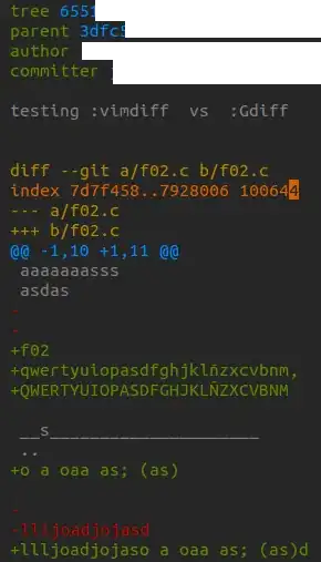
Here is a screen shot.

Daniel Lichtblau Wolfram Research

Answer 4

Mathematica isn't the best software for this, although it will work out.

http://demonstrations.wolfram.com/DrawingATriangle/ has source code for a really nice triangle, and following that example you can add a bisecting line to the code.

Answer 5

As already stated, Mathematica is not the best software for this. There are several better options that you can use, depending on your exact purpose. To generate such figures programatically, there are several languages especially adapted for such tasks. I would recommend to try eukleides or GCLC. If you have any experience with TeX/LaTeX, you may want to look at metapost or asymptote, or even a LaTeX package such as tkz-euklide.

If you on the other hand prefer to create you drawings in an interactive way, there are number of programs available. Search the web for "dynamic geometry software", you should get a number of hits. Of those I would most recommend geogebra.

Answer 6

I thought that I should really attempt this problem in Mathematica (only once I finished did I see Daniel's solution). It took me about half an hour - which is longer than my GeoGebra solution, despite the fact that I'd never used GeoGebra before.

The code is not as fast as it could be. This is because I was too lazy to code up proper code for finding intersections of lines and circles, so I just used the slower but more general FindInstance.

A quite comprehensive plane geometry package can be found as part of Eric Weinstein's MathWorld packages. It includes all the intersection, bisection etc... code that you could possibly want, but it would take a little bit of time to learn it all.

angleBisector[A_,{B_,C_}]:=Module[{ba=Norm[B-A],ca=Norm[C-A],m},
  m=A+((B-A)/ba+(C-A)/ca)]

intersect[Line[{A_,B_}],Line[{C_,D_}]]:=Module[{s,t},
  A + s(B-A)/.First@FindInstance[A + s(B-A) == C + t(D-C), {s,t}]]
intersect[Line[{A_,B_}],Circle[p0:{x0_,y0_},r_]]:=Module[{s,x,y},
  A + s(B-A)/.FindInstance[A + s(B-A) == {x,y} 
  && Norm[p0-{x,y}] == r, {s,x,y}, Reals, 2]]

Manipulate[Module[{OO,circ,tri,angB,int,mid,FF},
  OO=(AA+BB)/2;
  circ=Circle[OO,Norm[AA-BB]/2];
  tri=Line[{AA,BB,CC,AA}];
  angB=angleBisector[AA,{BB,CC}];
  int=intersect[Line[{BB,CC}],Line[{AA,angB}]];
  mid=(AA+int)/2;
  FF=intersect[Line[{CC,mid}],Circle[OO,Norm[AA-BB]/2]];
  Graphics[{PointSize[Large],Point[{OO,int,mid}],Point[FF],tri,circ,
    Line[{AA,AA+3(angB-AA)}],Line[{CC,CC+3(mid-CC)}],
    Text["A",AA,{2,-2}],Text["B",BB,{-2,-2}],Text["C",CC,{2,2}],
    Text["O",OO,{0,-2}],Text["D",int,{-2,-1}],Text["M",mid,{-2,-1}]},
    PlotRange->{{-2,2},{-2,2}}]],
  {{AA,{-1,1}},Locator},
  {{BB,{1,1}},Locator},
  {{CC,{0,-1}},Locator}]