Overlay raster plot using plot(...,add=T) leads to arbitrary misalignment of final plot

Question

I have found that when I try to overlay multiple rasters using plot(...,add=T) if I try to overlay more than 3 rasters together the subsequent plot does not align the rasters properly.

My original intent was to create a categorical map of modeled landcover where the darkness of the color representing a cover class varied wrt the certainty in our model projection. To do this, I created a simple script that would loop through each cover class and plot it (e.g., forest, green color on map) using a color gradient from grey (low certainty forest prediction) to full cover color (e.g., dark green for areas are strongly predicted). What I have found is that using this approach, after the 3rd cover is added to the plot, all subsequent rasters that are overlayed on the plot are arbitrarily misaligned. I have reversed the order of plotting of the cover classes and the same behavior is exhibited meaning it is not an issue with the individual cover class rasters. Even more puzzling in Rstudio, when I use the zoom button to closely inspect the final plot, the misalignment worsens.

Do you have any ideas of why this behavior exists? Most importantly, do you have any suggested solutions or workarounds?

The code and data on the link below has all of the behaviors described captured. https://dl.dropboxusercontent.com/u/332961/r%20plot%20raster%20add%20issue.zip Turn plot_gradient=F to see how if you just simply subset a same raster and add the subsets sequentially to the same plot you can replicate the issue. I have already tried setting the extent of the plot device plot(..., ext) but that did not work. I have also checked and the extent of each cover raster is the same.

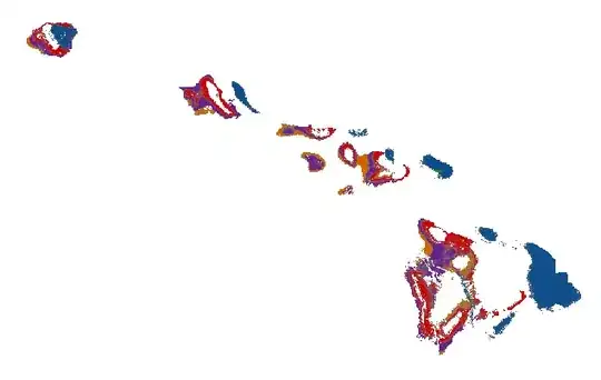
Below is the figure of the misaligned cover classes. plotting to jpeg device will result in a similar image (i.e., this is not an issue of Rstudio rendering). Strangely enough, if I zoom into the image using Rstudio, the misalignment is different For comparison, this is how the covers should align correctly in the landscape

library(raster)
library(colorRamps)
raster_of_classes=raster("C:/r plot raster add issue/raster_of_classes.tif")
raster_of_certainty_of_classes=raster("C:/r plot raster add issue/raster_of_certainty_of_classes.tif")
endCols=c("darkorchid4", "darkorange3", "red3", "green4", "dodgerblue4") #colors to be used in gradients for each class
classes=unique(raster_of_classes)
minVal=cellStats(raster_of_certainty_of_classes, min)
tmp_i=1
addPlot=F
plot_gradient=F #this is for debug only
#classes=rev(classes) #turn this off and on to see how last 2 classes are mis aligned, regardless of plotting order
for (class in classes){
  raster_class=raster_of_classes==class #create mask for individual class
  raster_class[raster_class==0]=NA #remove 0s from mask so they to do not get plotted
  if (plot_gradient){
    raster_of_certainty_of_class=raster_of_certainty_of_classes*raster_class #apply class mask to certainty map 
  }else{
    raster_of_certainty_of_class=raster_class #apply class mask to certainty map
  }
  endCol=endCols[tmp_i] #pick color for gradient
  col5 <- colorRampPalette(c('grey50', endCol))  
  if (plot_gradient){
    plot(raster_of_certainty_of_class, 
         col=col5(n=49), breaks=seq(minVal,1,length.out=50), #as uncertainty values range from 0 to 1 plot them with fixed range
         useRaster=T, axes=FALSE, box=FALSE, add=addPlot, legend=F)      
  }else{
    plot(raster_of_certainty_of_class, 
         col=endCol,       
         useRaster=T, axes=FALSE, box=FALSE, add=addPlot, legend=F)      
  }
  tmp_i=tmp_i+1
  addPlot=T #after plotting first class, all other classes are added
}

Answer 1

I had this problem too and solved it by calling the graphical parameters function, par(), with a subset of parameters, and most importantly, put the new=TRUE in the par() call, not the plot() call, before each additional plot() call. For example:

  png(fullname,
      width = 3000, 
      height= 3000)

  # original par() call
  par(mfrow=c(1,1), cex=3, mar=c(3,3,3,7), bg=bgcol, col=txtcol)

  # first plot
  plot(zreate,
       maxpixels=ncell(zreate),
       col=qcol,
       colNA=mapbg,
       xaxt='n',
       yaxt='n',
       ext=map_extent,
       breaks=tq,
       bty='n',
       legend=FALSE)

    #second plot and par() call
    par(mfrow=c(1,1), cex=3, mar=c(3,3,3,7), bg=bgcol, col=txtcol, new=TRUE)
    plot(rt,
         maxpixels=ncell(rt),
         col=dcol,
         legend=FALSE,
         xaxt='n',
         yaxt='n',
         ext=map_extent,
         bty='n')

    #third plot and par() call
    par(mfrow=c(1,1), cex=3, mar=c(3,3,3,7), bg=bgcol, col=txtcol, new=TRUE)
    plot(r0,
         maxpixels=ncell(r0),
         col="#9e9ac8",
         xaxt='n',
         yaxt='n',
         ext=map_extent, #PRENAFILTERING fix
         bty='n',
         legend=FALSE)

Answer 2

In December 2013, I posted a question about exactly this behavior to the R-sig-geo mailing list, and got no useful response (other than a confirmation that it also happens with R versions and OS's different than my own).

Here, for the record, is the reproducible example that I used to illustrate the issue. (See the linked question for some more explanation.)

library(maptools) ## Only needs to be installed for example data
library(raster)
library(rgeos)

## Create an example raster
p <- shapefile(system.file("shapes/co37_d90.shp", package="maptools"))
p <- p[31,]  ## A tall narrow county polygon
pr <- gDifference(gBuffer(p, width=.01), p)
r <- rasterize(pr, raster(extent(pr), ncol=100, nrow=100))

## These three are properly registered on one another
plot(r, col="yellow", legend=FALSE)
plot(r, col="green", legend=FALSE, add=TRUE)
plot(r, col="grey", legend=FALSE, add=TRUE)
## All subsequent "layers" are improperly shifted/skewed to right
plot(r, col="yellow", legend=FALSE, add=TRUE)
plot(r, col="blue", legend=FALSE, add=TRUE)
plot(r, col="red", legend=FALSE, add=TRUE)
plot(r, col="grey20", legend=FALSE, add=TRUE)
## Following the above, SpatialPolygons are also shifted/skewed
plot(p, border="red", lwd=2, add=TRUE)

Answer 3

I have run into the same problem and found an answer that is less of a hack than the previous answer. It follows the train of thought described by user "Dial".

The key is to use image(). But add in the argument maxpixels = ncell(x). This way, the resolution is maintained and pixel aggregation does not occur either as much or at all.

> x <- brick(image.path)
> plotRGB(x)

> image(brick.overlay, add = T, col = 'black', maxpixel = ncell(x))
> image(brick.overlay, add = T, col = 'yellow', maxpixel = ncell(x))

The "brick.overlay" would be some mask object, region of interest, or otherwise subsetted data where data is associated with those pixels and all other pixels are NA.

The brick.overlay object should have to have an implied extent based on total number of pixels where all non-interest pixels are NA.

This is hardly the most memory efficient way, but it's the one I know works.

If you use "Dial's" example, I think you would do:

image(r, col="yellow",  add=TRUE, maxpixels = ncell(r))

Answer 4

Interesting problem. As you likely know, image() doesn't seem to have the same issue but generally makes uglier maps, right?

    library(raster)
    library(rgeos)

    ## Create an example raster
    p <- shapefile(system.file("shapes/co37_d90.shp", package="maptools"))
    p <- p[31,]  ## A tall narrow county polygon
    pr <- gDifference(gBuffer(p, width=.01), p)
    r <- rasterize(pr, raster(extent(pr), ncol=100, nrow=100))


    ## These three are properly registered on one another
    image(r, col="yellow")
    image(r, col="green", add=TRUE)
    image(r, col="grey",  add=TRUE)
    ## All subsequent "layers" are also registered
    image(r, col="yellow",  add=TRUE)
    image(r, col="blue",  add=TRUE)
    image(r, col="red",  add=TRUE)
    image(r, col="grey20",  add=TRUE)
    ## Following the above, SpatialPolygons are no longer shifted/skewed
    plot(p, border="red", lwd=2, add=TRUE)