Artefacts from Riemann sum in scipy.signal.convolve

Question

Short summary: How do I quickly calculate the finite convolution of two arrays?

Problem description

I am trying to obtain the finite convolution of two functions f(x), g(x) defined by

To achieve this, I have taken discrete samples of the functions and turned them into arrays of length steps:

xarray = [x * i / steps for i in range(steps)]
farray = [f(x) for x in xarray]
garray = [g(x) for x in xarray]

I then tried to calculate the convolution using the scipy.signal.convolve function. This function gives the same results as the algorithm conv suggested here. However, the results differ considerably from analytical solutions. Modifying the algorithm conv to use the trapezoidal rule gives the desired results.

To illustrate this, I let

f(x) = exp(-x)
g(x) = 2 * exp(-2 * x)

the results are:

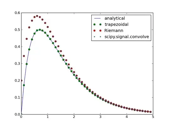
Here Riemann represents a simple Riemann sum, trapezoidal is a modified version of the Riemann algorithm to use the trapezoidal rule, scipy.signal.convolve is the scipy function and analytical is the analytical convolution.

Now let g(x) = x^2 * exp(-x) and the results become:

Here 'ratio' is the ratio of the values obtained from scipy to the analytical values. The above demonstrates that the problem cannot be solved by renormalising the integral.

The question

Is it possible to use the speed of scipy but retain the better results of a trapezoidal rule or do I have to write a C extension to achieve the desired results?

An example

Just copy and paste the code below to see the problem I am encountering. The two results can be brought to closer agreement by increasing the steps variable. I believe that the problem is due to artefacts from right hand Riemann sums because the integral is overestimated when it is increasing and approaches the analytical solution again as it is decreasing.

EDIT: I have now included the original algorithm 2 as a comparison which gives the same results as the scipy.signal.convolve function.

import numpy as np
import scipy.signal as signal
import matplotlib.pyplot as plt
import math

def convolveoriginal(x, y):
    '''
    The original algorithm from http://www.physics.rutgers.edu/~masud/computing/WPark_recipes_in_python.html.
    '''
    P, Q, N = len(x), len(y), len(x) + len(y) - 1
    z = []
    for k in range(N):
        t, lower, upper = 0, max(0, k - (Q - 1)), min(P - 1, k)
        for i in range(lower, upper + 1):
            t = t + x[i] * y[k - i]
        z.append(t)
    return np.array(z) #Modified to include conversion to numpy array

def convolve(y1, y2, dx = None):
    '''
    Compute the finite convolution of two signals of equal length.
    @param y1: First signal.
    @param y2: Second signal.
    @param dx: [optional] Integration step width.
    @note: Based on the algorithm at http://www.physics.rutgers.edu/~masud/computing/WPark_recipes_in_python.html.
    '''
    P = len(y1) #Determine the length of the signal
    z = [] #Create a list of convolution values
    for k in range(P):
        t = 0
        lower = max(0, k - (P - 1))
        upper = min(P - 1, k)
        for i in range(lower, upper):
            t += (y1[i] * y2[k - i] + y1[i + 1] * y2[k - (i + 1)]) / 2
        z.append(t)
    z = np.array(z) #Convert to a numpy array
    if dx != None: #Is a step width specified?
        z *= dx
    return z

steps = 50 #Number of integration steps
maxtime = 5 #Maximum time
dt = float(maxtime) / steps #Obtain the width of a time step
time = [dt * i for i in range (steps)] #Create an array of times
exp1 = [math.exp(-t) for t in time] #Create an array of function values
exp2 = [2 * math.exp(-2 * t) for t in time]
#Calculate the analytical expression
analytical = [2 * math.exp(-2 * t) * (-1 + math.exp(t)) for t in time]
#Calculate the trapezoidal convolution
trapezoidal = convolve(exp1, exp2, dt)
#Calculate the scipy convolution
sci = signal.convolve(exp1, exp2, mode = 'full')
#Slice the first half to obtain the causal convolution and multiply by dt
#to account for the step width
sci = sci[0:steps] * dt
#Calculate the convolution using the original Riemann sum algorithm
riemann = convolveoriginal(exp1, exp2)
riemann = riemann[0:steps] * dt

#Plot
plt.plot(time, analytical, label = 'analytical')
plt.plot(time, trapezoidal, 'o', label = 'trapezoidal')
plt.plot(time, riemann, 'o', label = 'Riemann')
plt.plot(time, sci, '.', label = 'scipy.signal.convolve')
plt.legend()
plt.show()

Thank you for your time!

Answer 1

or, for those who prefer numpy to C. It will be slower than the C implementation, but it's just a few lines.

>>> t = np.linspace(0, maxtime-dt, 50)
>>> fx = np.exp(-np.array(t))
>>> gx = 2*np.exp(-2*np.array(t))
>>> analytical = 2 * np.exp(-2 * t) * (-1 + np.exp(t))

this looks like trapezoidal in this case (but I didn't check the math)

>>> s2a = signal.convolve(fx[1:], gx, 'full')*dt
>>> s2b = signal.convolve(fx, gx[1:], 'full')*dt
>>> s = (s2a+s2b)/2
>>> s[:10]
array([ 0.17235682,  0.29706872,  0.38433313,  0.44235042,  0.47770012,
        0.49564748,  0.50039326,  0.49527721,  0.48294359,  0.46547582])
>>> analytical[:10]
array([ 0.        ,  0.17221333,  0.29682141,  0.38401317,  0.44198216,
        0.47730244,  0.49523485,  0.49997668,  0.49486489,  0.48254154])

largest absolute error:

>>> np.max(np.abs(s[:len(analytical)-1] - analytical[1:]))
0.00041657780840698155
>>> np.argmax(np.abs(s[:len(analytical)-1] - analytical[1:]))
6

Answer 2

Short answer: Write it in C!

Long answer

Using the cookbook about numpy arrays I rewrote the trapezoidal convolution method in C. In order to use the C code one requires three files (https://gist.github.com/1626919)

• The C code (performancemodule.c).
• The setup file to build the code and make it callable from python (performancemodulesetup.py).
• The python file that makes use of the C extension (performancetest.py)

The code should run upon downloading by doing the following

• Adjust the include path in performancemodule.c.

• Run the following

  python performancemodulesetup.py build python performancetest.py

You may have to copy the library file performancemodule.so or performancemodule.dll into the same directory as performancetest.py.

Results and performance

The results agree neatly with one another as shown below:

The performance of the C method is even better than scipy's convolve method. Running 10k convolutions with array length 50 requires

convolve (seconds, microseconds) 81 349969
scipy.signal.convolve (seconds, microseconds) 1 962599
convolve in C (seconds, microseconds) 0 87024

Thus, the C implementation is about 1000 times faster than the python implementation and a bit more than 20 times as fast as the scipy implementation (admittedly, the scipy implementation is more versatile).

EDIT: This does not solve the original question exactly but is sufficient for my purposes.