Bezier Curve Evaluation

Question

I am following this paper here using de Casteljau's Algorithm http://www.cgafaq.info/wiki/B%C3%A9zier_curve_evaluation and I have tried using the topic Drawing Bezier curves using De Casteljau Algorithm in C++ , OpenGL to help. No success.

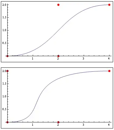
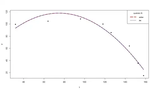
My bezier curves look like this when evaluated

As you can see, even though it doesn't work the wanted I wanted it to, all the points are indeed on the curve. I do not think that this algorithm is inaccurate for this reason.

Here are my points on the top curve in that image: (0,0) (2,0) (2,2) (4,2) The second curve uses the same set of points, except the third point is (0,2), that is, two units above the first point, forming a steeper curve.

Something is wrong. I should put in 0.25 for t and it should spit out 1.0 for the X value, and .75 should always return 3. Assume t is time. It should progress at a constant rate, yeah? Exactly 25% of the way in, the X value should be 1.0 and then the Y should be associated with that value.

Are there any adequate ways to evaluate a bezier curve? Does anyone know what is going on here?

Thanks for any help! :)

EDIT------

I found this book in a google search http://www.tsplines.com/resources/class_notes/Bezier_curves.pdf and here is the page I found on explicit / non-parametric bezier curves. They are polynomials represented as bezier curves, which is what I am going for here. Here is that page from the book:

Anyone know how to convert a bezier curve to a parametric curve? I may open a different thread now...

EDIT AGAIN AS OF 1 NOVEMBER 2011-------

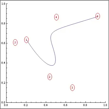
I've realized that I was only asking the question about half as clear as I should have. What I'm trying to build is like Maya's animation graph editor such as this http://www.youtube.com/watch?v=tckN35eYJtg&t=240 where the bezier control points that are used to modify the curve are more like tangent modifiers of equal length. I didn't remember them as being equal length, to be honest. By forcing a system like this, you can insure 100% that the result is a function and contains no overlapping segments.

I found this, which may have my answer http://create.msdn.com/en-US/education/catalog/utility/curve_editor

Answer 1

Here you can see the algorithm implemented in Mathematica following the nomenclature in your link, and your two plots:

(*Function Definitions*)

lerp[a_, b_, t_] := (1 - t) a + t b;
pts1[t_] := {
   lerp[pts[[1]], pts[[2]], t],
   lerp[pts[[2]], pts[[3]], t],
   lerp[pts[[3]], pts[[4]], t]};
pts2[t_] := {
   lerp[pts1[t][[1]], pts1[t][[2]], t],
   lerp[pts1[t][[2]], pts1[t][[3]], t]};
pts3[t_] := {
   lerp[pts2[t][[1]], pts2[t][[2]], t]};

(*Usages*)

pts = {{0, 0}, {2, 0}, {2, 2}, {4, 2}};
Framed@Show[ParametricPlot[pts3[t], {t, 0, 1}, Axes -> True], 
            Graphics[{Red, PointSize[Large], Point@pts}]]

pts = {{0, 0}, {2, 0}, {0, 2}, {4, 2}};
Framed@Show[ParametricPlot[pts3[t], {t, 0, 1}, Axes -> True], 
            Graphics[{Red, PointSize[Large], Point@pts}]]

BTW, the curves are defined by the following parametric equations, which are the functions pts3[t] in the code above:

c1[t_] := {2 t (3 + t (-3 + 2 t)), (* <- X component *)
                 2 (3 - 2 t) t^2}  (* <- Y component *)

and

c2[t_] := {2 t (3 + t (-6 + 5 t)), (* <- X component *)
               , 2 (3 - 2 t) t^2}  (* <- Y component *)

Try plotting them!

Taking any of these curve equations, and by solving a cubic polynomial you can in these cases get an expression for y[x], which is certainly not always possible. Just for you to get a flavor of it, from the first curve you get (C syntax):

y[x]= 3 - x - 3/Power(-2 + x + Sqrt(5 + (-4 + x)*x),1/3) + 
              3*Power(-2 + x + Sqrt(5 + (-4 + x)*x),1/3)

Try plotting it!

Edit

Just an amusement:

Mathematica is a quite powerful functional language, and in fact the whole algorithm can be expressed as a one liner:

f = Nest[(1 - t) #[[1]] + t #[[2]] & /@ Partition[#, 2, 1] &, #, Length@# - 1] &

Such as

f@{{0, 0}, {2, 0}, {0, 2}, {4, 2}}

gives the above results, but supports any number of points.

Let's try with six random points:

p = RandomReal[1, {6, 2}];
Framed@Show[
  Graphics[{Red, PointSize[Large], Point@p}],
  ParametricPlot[f@p, {t, 0, 1}, Axes -> True]]

Moreover, the same function works in 3D:

p = RandomReal[1, {4, 3}];
Framed@Show[
  Graphics3D[{Red, PointSize[Large], Point@p}],
  ParametricPlot3D[f[p], {t, 0, 1}, Axes -> True]]

Answer 2

A bezier curve can be solved by solving the following parametric equations for the x, y, and z coordinates (if it's just 2D, do only x and y):

Px = (1-t)^3(P1x) + 3t(1-t)^2(P2x) + 3t^2(1-t)(P3x) + t^3(P4x)
Py = (1-t)^3(P1y) + 3t(1-t)^2(P2y) + 3t^2(1-t)(P3y) + t^3(P4y)
Pz = (1-t)^3(P1z) + 3t(1-t)^2(P2z) + 3t^2(1-t)(P3z) + t^3(P4z)

You can also solve this by multiplying the matrix equation ABC = X where:

1. matrix A is a 1x4 matrix and represents the values of the powers of t
2. matrix B are the coefficients of the powers of t, and is a lower-triangular 4x4 matrix
3. matrix C is a 4x3 matrix that represents each of the four bezier points in 3D-space (it would be a 4x2 matrix in 2D-space)

This would look like the following:

(Update - the bottom left 1 ought to be a -1)

An important note in both forms of the equation (the parametric and the matrix forms) is that t is in the range [0, 1].

Rather than attempting to solve the values for t that will give you integral values of x and y, which is going to be time-consuming given that you're basically solving for the real root of a 3rd-degree polynomial, it's much better to simply create a small enough differential in your t value such that the difference between any two points on the curve is smaller than a pixel-value increment. In other words the distance between the two points P(t1) and P(t2) is such that it is less than a pixel value. Alternatively, you can use a larger differential in t, and simply linearly interpolate between P(t1) and P(t2), keeping in mind that the curve may not be "smooth" if the differential between P(t1) and P(t2) is not small enough for the given range of t from [0, 1].

A good way to find the necessary differential in t to create a fairly "smooth" curve from a visual standpoint is to actually measure the distance between the four points that define the bezier curve. Measure the distance from P1 to P2, P2, to P3, and P3 to P4. Then take the longest distance, and use the inverse of that value as the differential for t. You may still need to-do some linear interpolation between points, but the number of pixels in each "linear" sub-curve should be fairly small, and therefore the curve itself will appear fairly smooth. You can always decrease the differential value on t from this initial value to make it "smoother".

Finally, to answer your question:

Assume t is time. It should progress at a constant rate, yeah? Exactly 25% of the way in, the X value should be 1.0 and then the Y should be associated with that value.

No, that is not correct, and the reason is that the vectors (P2 - P1) and (P3 - P4) are not only tangent to the bezier curve at P1 and P4, but their lengths define the velocity along the curve at those points as well. Thus if the vector (P2 - P1) is a short distance, then that means for a given amount of time t, you will not travel very far from the point P1 ... this translates into the x,y values along the curve being packed together very closely for a given fixed differential of t. You are effectively "slowing down" in velocity as you move towards P1. The same effect takes place at P4 on the curve depending on the length of the vector (P3 - P4). The only way that the velocity along the curve would be "constant", and therefore the distance between any points for a common differential of t would be the same, would be if the lengths of all three segements (P2 - P1), (P3 - P2), and (P4 - P3) were the same. That would then indicate that there was no change in velocity along the curve.

Answer 3

It sounds like you actually just want a 1D cubic Bezier curve instead of the 2D that you have. Specifically, what you actually want is just a cubic polynomial segment that starts at 0 and goes up to 2 when evaluated over the domain of 0 to 4. So you could use some basic math and just find the polynomial:

f(x) = a + b*x + c*x^2 + d*x^3
f(0) = 0
f(4) = 2

That leaves two degrees of freedom.
Take the derivative of the function:

f'(x) = b + 2*c*x + 3*d*x^2

If you want it to be steep at the beginning and then level off at the end you might say something like:

f'(0) = 10
f'(4) = 0

Then we can plug in values. a and b come for free because we're evaluating at zero.

a = 0
b = 10

So then we have:

f(4) = 2 = 40 + c*16 + d*64
f'(4) = 0 = 10 + c*8 + d*48

That's a pretty easy linear system to solve. For completeness, we get:

16c + 64d = -38
 8c + 48d = -10

So-

1/(16*48 - 8*64)|48 -64||-38| = |c| = |-37/8 |
                |-8  16||-10|   |d|   |  9/16|

f(x) = 10*x - (37/8)*x^2 + (9/16)*x^3

If, instead, you decide that you want to use Bezier control points, just pick your 4 y-value control points and recognize that in order to get t in [0,1], you just have to say t=x/4 (remembering that if you also need derivatives, you'll have to do a change there too).

---

Added:

If you happen to know the points and derivatives you want to begin and end with, but you want to use Bezier control points P1, P2, P3, and P4, the mapping is just this (assuming a curve parametrized over 0 to 1):

P1 = f(0)
P2 = f'(0)/3 + f(0)
P3 = f(1) - f'(1)/3
P4 = f(1)

If, for some reason, you wanted to stick with your 2D Bezier control points and wanted to ensure that the x dimension advanced linearly from 0 to 2 as t advanced from 0 to 1, then you could do that with control points (0,y1) (2/3,y2) (4/3,y3) (2,y4). You can see that I just made the x dimension start at 0, end at 2, and have a constant slope (derivative) of 2 (with respect to t). Then you just make the y-coordinate be whatever you need it to be. The different dimensions are essentially independent of each other.

Answer 4

After all this time, I was looking for hermite curves. Hermites are good because in one dimension they're guaranteed to produce a functional curve that can be evaluated to an XY point. I was confusing Hermites with Bezier.

Answer 5

"Assume t is time."

This is the problem - t is not the time. The curve has it's own rate of change of t, depending on the magnitude of the tangents. Like Jason said, the distance between the consequent points must be the same in order of t to be the same as the time. This is exactly what the non-weighted mode (which is used by default) in the Maya's curve editor is. So this was a perfectly good answer for how to fix this issue. To make this work for arbitrary tangents, you must convert the time to t. You can find t by calculating the bezier equation in the x (or time) direction.

Px = (1-t)^3(P1x) + 3t(1-t)^2(P2x) + 3t^2(1-t)(P3x) + t^3(P4x)

Px is your time, so you know everything here, but t. You must solve a cubic equation to find the roots. There is a tricky part to find the exact root you need though. Then you solve the other equation to find Py (the actual value you are looking for), knowing now t:

Py = (1-t)^3(P1y) + 3t(1-t)^2(P2y) + 3t^2(1-t)(P3y) + t^3(P4y)

This is what the weighted curves in Maya are. I know the question is old, but I lost a whole day researching this simple thing, and nobody explains exactly what happens. Otherwise, the calculation process itself is written on many places, the Maya API manual for example. The Maya devkit also has a source code to do this.