Adding a trendline in basic R code (no GGPlot) for multiple plot graph of exponential and 2 factor polynomial curves

Question

I am trying to add trendlines to a multi-plot graph using basic R code. Could use some help to to add trendlines for non-linear functions, and am not sure if this is possible with basic R. I may need to upgrade my skillset to ggplot and thought I would check here first.

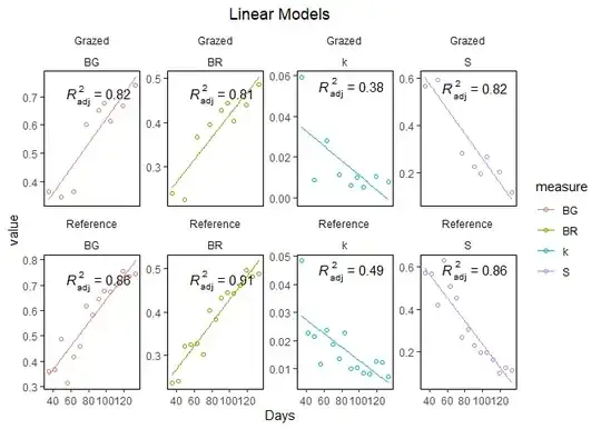
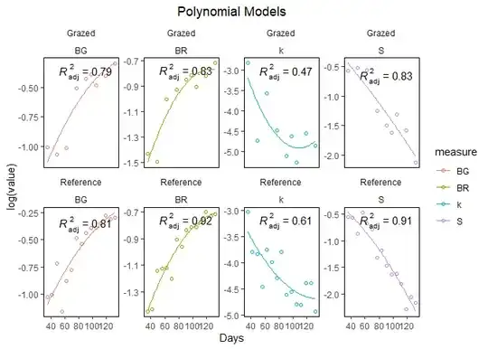
I have soil data for two locations, a reference site, and a site grazed by livestock. There are four litter decomposition metrics that I've tracked over time at each location: S, k, Bg and Br. The purpose of this experiment was to determine the shape of the decomposition curve for each metric. R2 analysis identified that S has best fit to an exponential model of decay, while k, Bg and Br are best fit to a 2 factor polynomial curve.

I'm trying to visualize the shapes of each best fit curve to each metric over time. I have tried to add trendlines but can't make anything work that isn't linear. I have tried different abline functions but am not sure this is the right approach. Thank you Allan Cameron for your response. I've edited this question to provide the full code for each of my models. I'm not sure how to upload my dataframe but have also provided some header data from my .csv.

Here is the R code that I've been working with so far:

# Create a new plot
plot.new()

# Set up multiple plots to visualize data (4 rows, 2 columns)
par(mfrow = c(1, 1))

# Plot S for each site

# Graph linear model of S for Reference against the number of 
# days in the ground
plot(soil_data$Days1, soil_data$S1, col = "darkgreen", xlab = "Days",
    ylab = "S", ylim = c(0, 0.7), las = 1,
   main = "Reference")

modelS1 <- lm(S1 ~ Days1, data = soil_data)
abline(modelS, col = "green")
legend(100, 0.70, bty="n", legend=c("R2 = 0.873"))
summary(modelS1)

# Graph linear model of S for Grazed against the number of 
# days in the ground
plot(soil_data$Days2, soil_data$S2, col = "darkgreen", xlab = "Days",
    ylab = "S", ylim = c(0, 0.7), las = 1,
     main = "Grazed")

modelS2 <- lm(S2 ~ Days2, data = soil_data)
abline(modelS2, col = "green")
legend(100, 0.70, bty="n", legend=c("R2 = 0.839"))
summary(modelS2)

# Graph linear model of S for Combined Sites against the 
# number of days in the ground
plot(soil_data$Days, soil_data$S, col = "darkblue", xlab = "Days",
    ylab = "S", ylim = c(0, 0.7), las = 1,
 main = "Combined")

modelS <- lm(S ~ Days, data = soil_data)
abline(modelS, col = "darkblue")
legend(100, 0.70, bty="n", legend=c("R2 = 0.857"))
summary(modelS)

# Plot linear model of k for each site 

# Graph linear model of k for Reference against the number of 
# days in the ground
plot(soil_data$Days1, soil_data$k1, col = "darkred", xlab = "Days",
 ylab = "k", ylim = c(0, 0.05), las = 1,
 main = "Reference")

modelk1 <- lm(k1 ~ Days1, data = soil_data)
abline(modelk1, col = "darkred")
legend("topright", bty="n", legend=c("R2 = 0.523"))
summary(modelk1)

# Graph linear model of k for Grazed against the # days in the ground
plot(soil_data$Days2, soil_data$k2, col = "darkred", xlab = "Days",
 ylab = "k", ylim = c(0, 0.05), las = 1,
 main = "Grazed")

modelk2 <- lm(k2 ~ Days2, data = soil_data)
abline(modelk2, col = "darkred")
legend("topright", bty="n", legend=c("R2 = 0.459"))
summary(modelk2)

# Graph linear model of k for Combined Sites against the # days 
plot(soil_data$Days, soil_data$k, col = "darkblue", xlab = "Days",
 ylab = "k", ylim = c(0, 0.05), las = 1,
 main = "Combined")

modelk <- lm(k ~ Days, data = soil_data)
abline(modelk, col = "darkblue")
legend("topright", bty="n", legend=c("R2 = 0.465"))
summary(modelk)

# Plot linear model of Bg for each site 

# Graph linear model of Bg for Reference against the number of days 
plot(soil_data$Days1, soil_data$BG1, col = "green", xlab = "Days",
 ylab = "Bg", ylim = c(0.3, 0.8), las = 1,
 main = "Reference")

modelBG1 <- lm(BG1 ~ Days1, data = soil_data)
abline(modelBG1, col = "green")
legend(100, 0.40, bty="n", legend=c("R2 = 0.873"))
summary(modelBG1)

# Graph linear model of Bg for Grazed against the number of days 
plot(soil_data$Days2, soil_data$BG2, col = "green", xlab = "Days",
 ylab = "Bg", ylim = c(0.3, 0.8), las = 1,
 main = "Grazed")

modelBG2 <- lm(BG2 ~ Days2, data = soil_data)
abline(modelBG2, col = "green")
legend(100, 0.40, bty="n", legend=c("R2 = 0.839"))
summary(modelBG2)

# Graph linear model of Bg for Combined Sites against # of days 
plot(soil_data$Days, soil_data$BG, col = "darkblue", xlab = "Days",
 ylab = "Bg", ylim = c(0.3, 0.8), las = 1,
 main = "Combined")

modelBG <- lm(BG ~ Days, data = soil_data)
abline(modelBG, col = "darkblue")
legend(100, 0.40, bty="n", legend=c("R2 = 0.857"))
summary(modelBG)

# Plot linear model of Br for each site

# Graph linear model of Br for reference against the # days 
plot(soil_data$Days1, soil_data$BR1, col = "darkred", xlab = "Days",
 ylab = "Br", ylim = c(0.2, 0.5), las = 1,
 main = "Reference")

modelBR1 <- lm(BR1 ~ Days1, data = soil_data)
abline(modelBR1, col = "darkred")
legend("bottomright", bty="n", legend=c("R2 = 0.921"))
summary(modelBR1)

# Graph linear model of Br for Grazed against the # of days 
plot(soil_data$Days2, soil_data$BR2, col = "darkred", xlab = "Days",
 ylab = "Br", ylim = c(0.2, 0.5), las = 1,
 main = "Grazed")

modelBR2 <- lm(BR2 ~ Days2, data = soil_data)
abline(modelBR2, col = "darkred")
legend("bottomright", bty="n", legend=c("R2 = 0.833"))
summary(modelBR2)

# Graph linear model of Br for Combined against the number of days 
plot(soil_data$Days, soil_data$BR, col = "darkblue", xlab = "Days",
 ylab = "Br", ylim = c(0.2, 0.5), las = 1,
 main = "Combined")

modelBR <- lm(BR ~ Days, data = soil_data)
abline(modelBR, col = "darkblue")
legend("bottomright", bty="n", legend=c("R2 = 0.885"))
summary(modelBR)

# EXPONENTIAL MODELS FOR EACH MATERIAL AND MEASURE 
# (log value of y axis)
# take the log of response variable, plot versus predictor 
# variable (days)
# method eg. https://www.statology.org/exponential-regression-in-r/

# Exponential model of S

# S Reference Exp
expSRef = lm(log(soil_data$S1) ~ soil_data$Days1)
summary(expSRef)

# S Grazed Exp
expSGraz = lm(log(soil_data$S2) ~ soil_data$Days2)
summary(expSGraz)

# S Combined Exp
expS = lm(log(soil_data$S) ~ soil_data$Days)
summary(expS)

# Exponential model of k for each site 

# k Reference Exp
expkRef = lm(log(soil_data$k1) ~ soil_data$Days1)
summary(expkRef)

# k Grazed Exp
expkGraz = lm(log(soil_data$k2) ~ soil_data$Days2)
summary(expkGraz)

# k Combined Exp
expk = lm(log(soil_data$k) ~ soil_data$Days)
summary(expk)

# Exponential model of Bg for each site 

# Bg Reference Exp
expBgRef = lm(log(soil_data$BG1) ~ soil_data$Days1)
summary(expBgRef)

# Bg Grazed Exp
expBgGraz = lm(log(soil_data$BG2) ~ soil_data$Days2)
summary(expBgGraz)

# Bg Combined Exp
expBg = lm(log(soil_data$BG) ~ soil_data$Days)
summary(expBg)

# Exponential model of Br for each site

# Br Reference Exp
expBrRef = lm(log(soil_data$BR1) ~ soil_data$Days1)
summary(expBrRef)

# Br Grazed Exp
expBrGraz = lm(log(soil_data$BR2) ~ soil_data$Days2)
summary(expBrGraz)

# Br Combined Exp
expBr = lm(log(soil_data$BR) ~ soil_data$Days)
summary(expBr)


# LOGARITHMIC MODELS FOR EACH MATERIAL AND MEASURE  
# (log value of x axis)
# https://www.statology.org/logarithmic-regression-in-r/

# Logarithmic model of S

# S Reference Log
logSRef = lm(log(soil_data$Days1) ~ soil_data$S1)
summary(logSRef)

# S Grazed Log
logSGraz = lm(log(soil_data$Days2) ~ soil_data$S2)
summary(logSGraz)

# S Combined Log
logS = lm(log(soil_data$Days) ~ soil_data$S)
summary(logS)


# Logarithmic model of k for each site 

# k Reference Log
logkRef = lm(log(soil_data$Days1) ~ soil_data$k1)
summary(logkRef)

# k Grazed Log
logkGraz = lm(log(soil_data$Days2) ~ soil_data$k2)
summary(logkGraz)

# k Combined Log
logk = lm(log(soil_data$Days) ~ soil_data$k)
summary(logk)

# Logarithmic model of Bg for each site 

# Bg Reference Log
logBgRef = lm(log(soil_data$Days1) ~ soil_data$BG1)
summary(logBgRef)

# Bg Grazed Log
logBgGraz = lm(log(soil_data$Days2) ~ soil_data$BG2)
summary(logBgGraz)

# Bg Combined Log
logBg = lm(log(soil_data$Days) ~ soil_data$BG)
summary(logBg)

# Logarithmic model of Br for each site

# Br Reference Log
logBrRef = lm(log(soil_data$Days1) ~ soil_data$BR1)
summary(logBrRef)

# Br Grazed Log
logBrGraz = lm(log(soil_data$Days2) ~ soil_data$BR2)
summary(logBrGraz)

# Br Combined Log
logBr = lm(log(soil_data$Days) ~ soil_data$BR)
summary(logBr)


# POLYNOMIAL MODEL OF EACH METRIC AND MEASURE - 2 dimensions

# Polynomial model of S

# S Reference Poly 2 dimensions
polySRef = lm(S1~poly(Days1, 2, raw = TRUE), data=soil_data)
summary(polySRef)

# S Grazed Poly 2 dimensions
polySGraz = lm(S2~poly(Days2, 2, raw = TRUE), data=soil_data)
summary(polySGraz)

# S Combined Poly 2 dimensions
polyS = lm(S~poly(Days, 2, raw = TRUE), data=soil_data)
summary(polyS)


# Polynomial model of k for each site 

# k Reference Poly 2 dimensions
polykRef = lm(k1~poly(Days1, 2, raw = TRUE), data=soil_data)
summary(polykRef)

# k Grazed Poly 2 dimensions
polykGraz = lm(k2~poly(Days2, 2, raw = TRUE), data=soil_data)
summary(polykGraz)

# k Combined Poly 2 dimensions
polyk = lm(k~poly(Days, 2, raw = TRUE), data=soil_data)
summary(polyk)

# Polynomial model of Bg for each site 

# Bg Reference Poly 2 dimensions
polyBgRef = lm(BG1~poly(Days1, 2, raw = TRUE), data=soil_data)
summary(polyBgRef)

# Bg Grazed Poly 2 dimensions
polyBgGraz = lm(BG2~poly(Days2, 2, raw = TRUE), data=soil_data)
summary(polyBgGraz)

# Bg Combined Poly 2 dimensions
polyBg = lm(BG~poly(Days, 2, raw = TRUE), data=soil_data)
summary(polyBg)

# Polynomial model of Br for each site

# Br Reference Poly 2 dimensions
polyBrRef = lm(BR1~poly(Days1, 2, raw = TRUE), data=soil_data)
summary(polyBrRef)

# Br Grazed Poly 2 dimensions
polyBrGraz = lm(BR2~poly(Days2, 2, raw = TRUE), data=soil_data)
summary(polyBrGraz)

# Br Combined Poly 2 dimensions
polyBr = lm(BR~poly(Days, 2, raw = TRUE), data=soil_data)
summary(polyBr)


# Summary R squared data for each model

# LINEAR
summary(modelS1)$r.squared
summary(modelS2)$r.squared
summary(modelS)$r.squared
summary(modelk1)$r.squared
summary(modelk2)$r.squared
summary(modelk)$r.squared
summary(modelBG1)$r.squared
summary(modelBG2)$r.squared
summary(modelBG)$r.squared
summary(modelBR1)$r.squared
summary(modelBR2)$r.squared
summary(modelBR)$r.squared

# EXPONENTIAL
summary(expSRef)$r.squared
summary(expSGraz)$r.squared
summary(expS)$r.squared
summary(expkRef)$r.squared
summary(expkGraz)$r.squared
summary(expk)$r.squared
summary(expBgRef)$r.squared
summary(expBgGraz)$r.squared
summary(expBg)$r.squared
summary(expBrRef)$r.squared
summary(expBrGraz)$r.squared
summary(expBr)$r.squared

# LOGARITHMIC 
summary(logSRef)$r.squared
summary(logSGraz)$r.squared
summary(logS)$r.squared
summary(logkRef)$r.squared
summary(logkGraz)$r.squared
summary(logk)$r.squared
summary(logBgRef)$r.squared
summary(logBgGraz)$r.squared
summary(logBg)$r.squared
summary(logBrRef)$r.squared
summary(logBrGraz)$r.squared
summary(logBr)$r.squared

# POLYNOMIAL - 2 dimensions
summary(polySRef)$r.squared
summary(polySGraz)$r.squared
summary(polyS)$r.squared
summary(polykRef)$r.squared
summary(polykGraz)$r.squared
summary(polyk)$r.squared
summary(polyBgRef)$r.squared
summary(polyBgGraz)$r.squared
summary(polyBg)$r.squared
summary(polyBrRef)$r.squared
summary(polyBrGraz)$r.squared
summary(polyBr)$r.squared

# Create combined dataset of S, k, Br, Bg, with 
# different shapes for each site

# Create a new plot
plot.new()

# Set up multiple plots to visualize data (4 rows, 2 columns)
par(mfrow = c(2, 2))

# Graph linear model of S for Combined Sites against # days 

plot(soil_data$Days[soil_data$Type == "Grazed"], 
soil_data$S[soil_data$Type == "Grazed"], 
 pch = 16, cex = 1, col = "darkblue", ylim = c(0, 0.7), 
xlab = "Days", ylab = "S", main = "S")
points(soil_data$Days[soil_data$Type == "Reference"], 
soil_data$S[soil_data$Type == "Reference"], 
   pch = 17, cex = 1, col = "darkred")
# this abline function is giving a straight line and 
# not the actual model, does the exp not make 
# an exponential trendline? 
abline(expSGraz, col = "darkblue")
abline(expSRef, col = "darkred")
legend("topright", legend = unique(soil_data$Type), pch = c(16, 17),
   col = c("darkblue", "darkred"), cex = 0.8, title = "Data Type")


# Now for k

plot(soil_data$Days[soil_data$Type == "Grazed"], 
soil_data$k[soil_data$Type == "Grazed"], 
 pch = 16, cex = 1, col = "darkblue", xlab = "Days", 
ylab = "k", main = "k")
points(soil_data$Days[soil_data$Type == "Reference"],
soil_data$k[soil_data$Type == "Reference"], 
   pch = 17, cex = 1, col = "darkred")
# this abline function is giving a straight line and 
# not the actual model 
abline(polykGraz, col = "darkblue")
abline(polykRef, col = "darkred")
legend("topright", legend = unique(soil_data$Type), pch = c(16, 17),
   col = c("darkblue", "darkred"), cex = 0.8, title = "Data Type")

# Bg

plot(soil_data$Days[soil_data$Type == "Grazed"],
soil_data$BG[soil_data$Type == "Grazed"], 
 pch = 16, cex = 1, col = "darkblue", xlab = "Days", 
ylab = "Bg", main = "Bg")
points(soil_data$Days[soil_data$Type == "Reference"],
soil_data$BG[soil_data$Type == "Reference"], 
   pch = 17, cex = 1, col = "darkred")
# this abline function is giving a straight line and 
# not the actual model 
abline(polyBgGraz, col = "darkblue")
abline(polyBgRef, col = "darkred")
legend("topleft", legend = unique(soil_data$Type), pch = c(16, 17),
   col = c("darkblue", "darkred"), cex = 0.8, title = "Data Type")

#Br

plot(soil_data$Days[soil_data$Type == "Grazed"],
soil_data$BR[soil_data$Type == "Grazed"], 
 pch = 16, cex = 1, col = "darkblue", xlab = "Days", 
ylab = "Br", main = "Br")
points(soil_data$Days[soil_data$Type == "Reference"],
soil_data$BR[soil_data$Type == "Reference"], 
   pch = 17, cex = 1, col = "darkred")
# this abline function is giving a straight line 
# and not the actual model 
abline(polyBrGraz, col = "darkblue")
abline(polyBrRef, col = "darkred")

legend("topleft", legend = unique(soil_data$Type), pch = c(16, 17),
   col = c("darkblue", "darkred"), cex = 0.8, title = "Data Type")

Data

dput(soil_data)
structure(list(Site = c(23L, 19L, 18L, 16L, 20L, 17L, 21L, 22L, 
24L, 6L, 7L, 2L, 5L, 3L, 12L, 13L, 8L, 14L, 9L, 15L, 4L, 1L, 
10L, 11L), Type = c("Grazed", "Grazed", "Grazed", "Grazed", "Grazed", 
"Grazed", "Grazed", "Grazed", "Grazed", "Reference", "Reference", 
"Reference", "Reference", "Reference", "Reference", "Reference", 
"Reference", "Reference", "Reference", "Reference", "Reference", 
"Reference", "Reference", "Reference"), Days = c(35L, 49L, 63L, 
77L, 91L, 98L, 105L, 119L, 133L, 35L, 42L, 49L, 56L, 63L, 70L, 
77L, 84L, 91L, 98L, 105L, 112L, 119L, 126L, 133L), S = c(0.566, 
0.593, 0.57, 0.285, 0.225, 0.197, 0.269, 0.205, 0.119, 0.573, 
0.566, 0.42, 0.628, 0.507, 0.455, 0.268, 0.306, 0.231, 0.196, 
0.198, 0.164, 0.101, 0.127, 0.114), k = c(0.0591, 0.0089, 0.0281, 
0.0113, 0.0061, 0.0099, 0.0052, 0.0106, 0.0079, 0.0484, 0.0227, 
0.0216, 0.0116, 0.0237, 0.0186, 0.0136, 0.0227, 0.01, 0.0105, 
0.0083, 0.0082, 0.0125, 0.0124, 0.0072), BG = c(0.365, 0.343, 
0.362, 0.602, 0.653, 0.676, 0.615, 0.669, 0.742, 0.359, 0.365, 
0.488, 0.313, 0.415, 0.459, 0.616, 0.584, 0.647, 0.677, 0.676, 
0.704, 0.757, 0.735, 0.746), BR = c(0.239, 0.225, 0.366, 0.395, 
0.428, 0.443, 0.403, 0.439, 0.486, 0.235, 0.239, 0.32, 0.325, 
0.327, 0.301, 0.404, 0.383, 0.433, 0.444, 0.443, 0.461, 0.496, 
0.482, 0.489), Days2 = c(35L, 49L, 63L, 77L, 91L, 98L, 105L, 
119L, 133L, NA, NA, NA, NA, NA, NA, NA, NA, NA, NA, NA, NA, NA, 
NA, NA), S2 = c(0.566, 0.593, 0.57, 0.285, 0.225, 0.197, 0.269, 
0.205, 0.119, NA, NA, NA, NA, NA, NA, NA, NA, NA, NA, NA, NA, 
NA, NA, NA), k2 = c(0.0591, 0.0089, 0.0281, 0.0113, 0.0061, 0.0099, 
0.0052, 0.0106, 0.0079, NA, NA, NA, NA, NA, NA, NA, NA, NA, NA, 
NA, NA, NA, NA, NA), BG2 = c(0.365, 0.343, 0.362, 0.602, 0.653, 
0.676, 0.615, 0.669, 0.742, NA, NA, NA, NA, NA, NA, NA, NA, NA, 
NA, NA, NA, NA, NA, NA), BR2 = c(0.239, 0.225, 0.366, 0.395, 
0.428, 0.443, 0.403, 0.439, 0.486, NA, NA, NA, NA, NA, NA, NA, 
NA, NA, NA, NA, NA, NA, NA, NA), Days1 = c(NA, NA, NA, NA, NA, 
NA, NA, NA, NA, 35L, 42L, 49L, 56L, 63L, 70L, 77L, 84L, 91L, 
98L, 105L, 112L, 119L, 126L, 133L), S1 = c(NA, NA, NA, NA, NA, 
NA, NA, NA, NA, 0.573, 0.566, 0.42, 0.628, 0.507, 0.455, 0.268, 
0.306, 0.231, 0.196, 0.198, 0.164, 0.101, 0.127, 0.114), k1 = c(NA, 
NA, NA, NA, NA, NA, NA, NA, NA, 0.0484, 0.0227, 0.0216, 0.0116, 
0.0237, 0.0186, 0.0136, 0.0227, 0.01, 0.0105, 0.0083, 0.0082, 
0.0125, 0.0124, 0.0072), BG1 = c(NA, NA, NA, NA, NA, NA, NA, 
NA, NA, 0.359, 0.365, 0.488, 0.313, 0.415, 0.459, 0.616, 0.584, 
0.647, 0.677, 0.676, 0.704, 0.757, 0.735, 0.746), BR1 = c(NA, 
NA, NA, NA, NA, NA, NA, NA, NA, 0.235, 0.239, 0.32, 0.325, 0.327, 
0.301, 0.404, 0.383, 0.433, 0.444, 0.443, 0.461, 0.496, 0.482, 
0.489)), class = "data.frame", row.names = c(NA, -24L))

Hi EBH. Welcome to Stack Overflow. It's going to be difficult to give you an answer with the information you have provided. We don't have `soil_data`, nor the code you used to create your models, so we cannot test or verify solutions. As a result, any code we offer could be wide of the mark and there is no way we can _demonstrate_ that it works. Please make your question _reproducible_. If you [edit] your question to include the output from `soil_data`, and the code used to generate your models, it will be easy to help. Without that, we can only give vague guidance in the comments. Thanks. — Allan Cameron, Aug 28 '23 at 20:36
Thank you @AllanCameron! I have updated the question. Please let me know if this is enough information to support a response. Clearly I'm new to this :| — EBH, Aug 28 '23 at 23:02
thank you. But can you please include the data as actual text that we can copy-paste into our consoles (perhaps the output from `dput(soil_data)`? Obviously, we can't run your code with a _picture_ of the data - we need the data itself (unless someone decides to transcribe your picture back into data, but this seems like an unreasonable thing to expect!) — Allan Cameron, Aug 28 '23 at 23:20
Thank you for the suggested prompt to pull the data out into this form. I've added it to the question - let me know if this works — EBH, Aug 28 '23 at 23:37

jpsmith · Answer 1 · 2023-08-29T12:56:30.533

In base R, you could substantially shorten the code needed for modeling and plotting by using list structures. I agree with @Allan Cameron that sometimes ggplot is better, but this could also be done in ~ 10 lines of code in Base R. Much like his excellent ggplot answer, I would convert to long format. Using these "long" data, you can run the model and store each value in a list using lapply then plot using sapply:

mdl <- lapply(unique(soil_data_long$measure), 
              function(x) lm(value ~ Days, data = soil_data_long[soil_data_long$measure == x,]))
names(mdl) <- unique(soil_data_long$measure)
par(mfrow = c(2,2))
sapply(unique(soil_data_long$measure), function(x){
  plot(value ~ Days, data = soil_data_long[soil_data_long$measure == x, ], 
       pch = 17, col = as.factor(Type), main = x)
  abline(mdl[[x]], col = "grey")
  legend(ifelse(x %in% c("S", "k"), "topright", "topleft"), c("Grazed", "Refernce"), pch = 17, col = 1:2, bty = "n")
  })

Here, the mdl uses lapply to run the model for each unique value of measure and then names them accordingly. We then set the par and use sapply to "loop" over each value of measure to create four different plots.

Note that I used Allan's code for converting to long:

soil_data_long <- soil_data %>%
  select(Site:BR) %>%
  pivot_longer(S:BR, names_to = 'measure')

Very nice looking plots they are too. I think the OP was specifically asking about adding lines for the polynomial and exponential models. I guess these could be added using `predict` directly rather than `abline` — Allan Cameron, Aug 29 '23 at 13:33
As yes, thank you @AllanCameron for that clarification - can use `predict` or something like `mdl[[x]]$fitted.values` (after running the exp and poly models) in `lines` instead of `abline` - will update when I have a bit more free time. — jpsmith, Aug 29 '23 at 14:09

score 1 · Answer 2 · answered Aug 29 '23 at 12:15

I understand you want to keep things in base R, but you are making things incredibly difficult for yourself here. To get the plots you want, you have written over 450 lines of code and have a vast number of variables polluting your global workspace.

Starting with your data, it is in a strange format. The y variable columns are repeated twice with NA values in an attempt to try to help you subgroup. This just makes things harder.

What I would suggest is selecting only the columns you need, and pivoting the y variables so that your data is in this format for plotting:

library(tidyverse)
library(ggpubr)

soil_data_long <- soil_data %>%
  select(Site:BR) %>%
  pivot_longer(S:BR, names_to = 'measure')

soil_data_long
#> # A tibble: 96 x 5
#>     Site Type    Days measure  value
#>    <int> <chr>  <int> <chr>    <dbl>
#>  1    23 Grazed    35 S       0.566 
#>  2    23 Grazed    35 k       0.0591
#>  3    23 Grazed    35 BG      0.365 
#>  4    23 Grazed    35 BR      0.239 
#>  5    19 Grazed    49 S       0.593 
#>  6    19 Grazed    49 k       0.0089
#>  7    19 Grazed    49 BG      0.343 
#>  8    19 Grazed    49 BR      0.225 
#>  9    18 Grazed    63 S       0.57  
#> 10    18 Grazed    63 k       0.0281
#> # ... with 86 more rows

Now you can plot all your linear models using only 12 lines of code

ggplot(soil_data_long, aes(Days, value, color = measure)) +
  geom_point(shape = 21) +
  stat_regline_equation(aes(label = after_stat(adj.rr.label)),
                        color = 'black', label.x.npc = 0.95,
                        label.y.npc = 0.95, hjust = 1) +
  geom_smooth(method = 'lm', formula = y ~ x, se = FALSE, linewidth = 0.5) +
  facet_wrap(Type ~ measure, ncol = 4, scales = 'free_y') +
  theme_classic() +
  theme(panel.border = element_rect(fill = NA),
        strip.background = element_blank(),
        plot.title = element_text(hjust = 0.5)) +
  ggtitle('Linear Models')

And similarly, your exponential models are just:

ggplot(soil_data_long, aes(Days, log(value), color = measure)) +
  geom_point(shape = 21) +
  stat_regline_equation(aes(label = after_stat(adj.rr.label)),
                        color = 'black', label.x.npc = 0.95,
                        label.y.npc = 0.95, hjust = 1) +
  geom_smooth(method = 'lm', formula = y ~ x, se = FALSE, linewidth = 0.5) +
  facet_wrap(Type ~ measure, ncol = 4, scales = 'free_y') +
  scale_y_continuous(breaks = log(seq(0.3, 0.8, 0.1)),
                     labels = ~exp(.x)) +
  labs(y = 'Value') +
  theme_classic() +
  theme(panel.border = element_rect(fill = NA),
        strip.background = element_blank(),
        plot.title = element_text(hjust = 0.5)) +
  coord_trans(y = 'exp') +
  ggtitle('Exponential Models')

And your poynomial models are just:

ggplot(soil_data_long, aes(Days, log(value), color = measure)) +
  geom_point(shape = 21) +
  stat_regline_equation(aes(label = after_stat(adj.rr.label)),
                        color = 'black', label.x.npc = 0.95,
                        label.y.npc = 0.95, hjust = 1,
                        formula =  y ~ poly(x, 2, raw = TRUE)) +
  geom_smooth(method = 'lm', formula = y ~ poly(x, 2, raw = TRUE), se = FALSE, 
              linewidth = 0.5) +
  facet_wrap(Type ~ measure, ncol = 4, scales = 'free_y') +
  theme_classic() +
  theme(panel.border = element_rect(fill = NA),
        strip.background = element_blank(),
        plot.title = element_text(hjust = 0.5)) +
  ggtitle('Polynomial Models')

Note that you only have two variables in your global workspace (your original and long-format data frames), and that your plots are easily and endlessly customizable with reusable code.

If you want to stick to base R plots, you can still do it, but I would stick to using the long-format data and using the split-lapply paradigm to plot rather than repeating yourself endlessly.

^{Created on 2023-08-29 with reprex v2.0.2}

I am beyond words and feel practically tearful with gratitude. R has been a challenge for me to learn, and I felt nervous stepping into this space with my very first question. Your incredibly thoughtful, clear, and detailed instructions are a gift. Thank you. I will make some (significant) adjustments to my code and thank you again for your support. — EBH, Aug 29 '23 at 15:13
how would I display the non-adjusted r squared values on these graphs? I tried after_stat(rsquared.label), but received an error message. — EBH, Sep 02 '23 at 16:56
I think it's `after_stat(rr.label)`. Look in `?stat_regline_equation` where it will tell you. — Allan Cameron, Sep 02 '23 at 18:55

score -1 · Answer 3 · answered Aug 29 '23 at 10:55

to be able to plot a trendline on your graphs shouldn't be too difficult.

You have created the linear models.

Use:

 coef(modelBG1)[1] for the intercept
 coef(modelBG1)[2] for the slope


 modelBG1 <- lm(BG1 ~ Days1, data = soil_data) # First the linear model

 plot(soil_data$Days1, soil_data$BG1, col = "green", xlab = "Days",
 ylab = "Bg", ylim = c(0.3, 0.8), las = 1, main = "Reference")
 # then the plot

 # then the abline or trend line 
 abline(coef(modelBG1)[1], coef(modelBG1)[2] , col = "green")

The above should give you the trend line where you will have gotten the coefficients from your linear models.

Hope this helps

Have you tested this code? It doesn't work properly – jpsmith Aug 29 '23 at 13:16 — jpsmith, Aug 29 '23 at 13:16

Adding a trendline in basic R code (no GGPlot) for multiple plot graph of exponential and 2 factor polynomial curves

3 Answers3