Is there a way in R i can create a new polygon (representing a certain constant value) based on two polygons representing 2 different constant values

Question

I have two polygons, an outer polygon and an inner polygon
The inner polygon is a polygon pol1 (red) for a parameter with a value = 10
The outer polygon is a polygon pol2 (blue) for a parameter with a value = 20
I need to draw a polygon for a value = 13 that would lie somewhere between pol1 and pol2
This is almost like buffering but not quite since buffering would only give me a constant distance.This is some sort of interpolation.
I think the solution would be like calculating distances from the odes in the inner polygon pol1 to the nearest edge of pol2
Then interpolating the distance for value = 13 for each node.
Then calculate the new points for a polygon pol3 for value= 13.
I could tediously try to code this but i imagine there may be a quicker/simpler solution Is there any tool that can help me to solve this. I would like Something that can be used with sf objects in R.

The code below is just for producing pol1 and pol2 which I hope someone can use to create a solution.

(In reality i have a more complex sf objects read from .shp files so I am thankful if you have example with such files )

 library(sf)


    #polygon1 value=10
    lon = c(21, 22,23,24,22,21)
    lat = c(1,2,1,2,3,1)
    Poly_Coord_df = data.frame(lon, lat)
    pol1 = st_polygon(
        list(
            cbind(
                Poly_Coord_df$lon,
                Poly_Coord_df$lat)
        )
    )
    
    
    
    #polygon2 value =20
    lon = c(21, 20,22,25,22,21)
    lat = c(0,3,5,4,-3,0)
    Poly_Coord_df = data.frame(lon, lat)
    pol2 = st_polygon(
        list(
            cbind(
                Poly_Coord_df$lon,
                Poly_Coord_df$lat)
        )
    )
    
    
    plot(pol2,border="blue")
    plot(pol1,border="red",add=T)

# How to create pol3 with value = 13?

It looks like you'll want to interpolate some [contour lines](https://mgimond.github.io/Spatial/interpolation-in-r.html), adding 20 to your first Poly_coord_df$elev <- 20, and 10 to the other. — Chris, Aug 17 '23 at 01:37

SamR · Answer 1 · 2023-08-17T21:35:40.490

As you say, this is a lot like buffering. It seems to me that we can approach it as creating a buffer around the inner polygon of whatever size your value is, and clipping that buffer to ensure it is never outside the outer polygon.

I've defined a function to do this, interpolate_polygon(). It first uses st_buffer() and then st_intersection() with the outer polygon for the clipping. You can plot the polygons created for selected values like this (original polygons red and blue, interpolated polygon is green):

vals_to_interpolate <- c(11, 13, 15, 17)
par(mfrow = c(2, 2))
for (val in vals_to_interpolate) {
    plot(pol2, border = "blue", main = sprintf("value: %s", val), cex.main = 3, lwd = 3)
    plot(pol1, border = "red", , lwd = 3, add = T)
    plot(interpolate_polygon(pol2, pol1, val),
        border = "green", , lwd = 3, add = T
    )
}

Function definition

Here is the definition of interpolate_polygon().

interpolate_polygon <- function(
    p_outer, p_inner, scale_val = 15,
    p_inner_val = 10, p_outer_val = 20,
    outer_buffer = 0.95) {
    # Just return outer polygon if you scale
    # all the way up

    if (scale_val == p_outer_val) {
        return(p_outer)
    }

    # Create a polygon that the inner polygon
    # can never extend past
    p_outer_scaled <- p_outer * outer_buffer
    p_outer_scaled <- p_outer_scaled - st_centroid(p_outer_scaled) + st_centroid(p_outer)

    p_inner_range <- as.matrix(p_inner) |>
        apply(2, range)

    p_outer_range <- as.matrix(p_outer) |>
        apply(2, range)

    max_stretch <- max(abs(p_outer_range - p_inner_range))

    # Create a buffer of appropriate size
    # cubic scaling seems to work
    buffer_val <- scales::rescale(
        scale_val^3,
        c(0, max_stretch),
        c(p_inner_val^3, p_outer_val^3)
    )

    p_scaled <- st_intersection(
        st_buffer(p_inner, buffer_val, joinStyle = "MITRE"),
        p_outer_scaled
    )

    p_scaled
}

This is a good answer but introduces some subjectivity on the outer boundary of the result due to a constat outer_buffer. You provide a good rough estimate. The the answer from @margusl works better for my kind of data although it provides some challenges with respect to speed if the raster is large. Thanks a lot. I have learnt alot from your approach and have a couple of ways i will use this. I feel through that your solution could work well if the outer_buffer is not set at a constant 0.95 but varied based on the and also if segmentizing can be added before buffering. — jjunju, Aug 21 '23 at 11:42
on second thought (after trial and error) i see that this solution creates a constat buffer based on scaling the values and then clipping. I am now of the view that this requirs substanstial modification in order to attain the result needed. — jjunju, Aug 21 '23 at 13:14
@jjunju are you referring to the buffer created in `p_outer_scaled` or the one created in `p_scaled`? The former is constant but that shouldn't matter - it's to stop the inner polygon extending outside the outer polygon. You could get rid of it if you want or just make it `p_outer`. The latter is not constant - you might want to play around with the scaling though. I made it cubic because it worked in your example, where there's a lot of space for the shape to extend on the y-axis but not much on the x-axis. I don't know what your real data looks like, but yes it may require some modification. — SamR, Aug 21 '23 at 13:49
even for p_scaled the buffer is a constant valuye around the entire polygon. i.e buffer_val though varies with scale_val but still leads to a constat buffer around the polygon. That is what i meant by constant buffer distance. it doesnt vary by node or line segment. — jjunju, Aug 21 '23 at 17:57

margusl · Accepted Answer · 2023-08-21T15:07:24.357

One option is to go through inverse distance weighted interpolation and "contour" the resulting raster. For idw to work, we first need a set of locations and a grid that defines resulting locations. For input locations we'll first segementize polygon lines so we would have bit more than just corner locations, then cast to POINTs. For the grid we'll first build a polygon that covers interpolation area and input polygon lines; this will be turned into stars raster. This also defines idw() output objects, which we can pass to stars::st_contour() to get polygons or linestings.

library(sf)
#> Linking to GEOS 3.9.3, GDAL 3.5.2, PROJ 8.2.1; sf_use_s2() is TRUE
library(stars)
#> Loading required package: abind
library(gstat)
library(ggplot2)

# inner polygon, value = 10
pol1 <- structure(list(structure(c(21, 22, 23, 24, 22, 21, 1, 2, 1, 2, 3, 1), 
                                 dim = c(6L, 2L))), class = c("XY", "POLYGON", "sfg"))
# outer polygon, value = 20
pol2 <- structure(list(structure(c(21, 20, 22, 25, 22, 21, 0, 3, 5, 4, -3, 0), 
                                 dim = c(6L, 2L))), class = c("XY", "POLYGON", "sfg"))

# sf object with value attributes
poly_sf <- st_sf(geometry = st_sfc(pol1, pol2), value = c(10, 20))

# mask for interpolation zone, polygon with hole, buffered
mask_sf <- st_difference(pol2, pol1) |> st_buffer(.1)

# points along LINESTRING, first segmentize so we would not end up with just 
# corner points
points_sf <- poly_sf |>
  st_segmentize(.1) |>
  st_cast("POINT")
#> Warning in st_cast.sf(st_segmentize(poly_sf, 0.1), "POINT"): repeating
#> attributes for all sub-geometries for which they may not be constant

# stars raster that defines interpolated output raster
grd <- st_bbox(mask_sf) |>
  st_as_stars(dx = .05) |>
  st_crop(mask_sf)


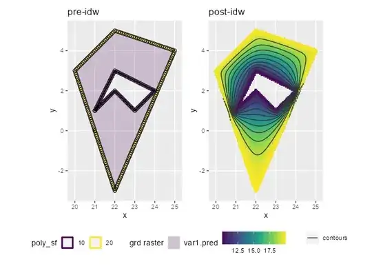
p1 <- ggplot() +
  geom_stars(data = grd, aes(fill = as.factor(values))) +
  geom_sf(data = poly_sf, aes(color = as.factor(value)), fill = NA, linewidth = 1, alpha = .5) +
  geom_sf(data = points_sf, shape = 1, size = 2) +
  scale_fill_viridis_d(na.value = "transparent", name = "grd raster", alpha = .2) +
  scale_color_viridis_d(name = "poly_sf") +
  theme(legend.position = "bottom") +
  ggtitle("pre-idw")

# inverse distance weighted interpolation of points on polygon lines,
# play around with idp (inverse distance weighting power) values, 2 is default
idw_stars <- idw(value ~ 1, points_sf, grd, idp = 2)
#> [inverse distance weighted interpolation]

# sf countour lines from raster
contour_sf <- idw_stars |> 
  st_contour(contour_lines = TRUE, breaks = 11:19)
names(contour_sf)[1] <- "value"

p2 <- ggplot() +
  geom_stars(data = idw_stars) +
  geom_sf(data = contour_sf, aes(color = "countours")) +
  scale_fill_viridis_c(na.value = "transparent") +
  scale_color_manual(values = c(countours = "grey20"), name = NULL) +
  theme(legend.position = "bottom") +
  ggtitle("post-idw")

patchwork::wrap_plots(p1,p2)


# combine interpolated contour(s) with input sf
out_sf <- contour_sf[contour_sf$value == 13, ] |> 
  st_polygonize() |> 
  st_collection_extract("POLYGON") |> 
  rbind(poly_sf)

Resulting sf object:

out_sf
#> Simple feature collection with 3 features and 1 field
#> Geometry type: POLYGON
#> Dimension:     XY
#> Bounding box:  xmin: 20 ymin: -3 xmax: 25 ymax: 5
#> CRS:           NA
#>    value                       geometry
#> 25    13 POLYGON ((22.975 0.8220076,...
#> 1     10 POLYGON ((21 1, 22 2, 23 1,...
#> 2     20 POLYGON ((21 0, 20 3, 22 5,...

# reorder for plot
out_sf$value <- as.factor(out_sf$value)
out_sf <- out_sf[rev(rank(st_area(out_sf))),] 
plot(out_sf)

Edit: other interpolation methods

IDW is just one of many interpolations methods; there's a good chance that some others are either faster and/or deliver more suitable results so it would probably be a good idea to look into Kriging methods (same gstat package) and maybe few others. E.g. one super-simple approach would be k-Nearest Neighbour Classification to detect the distance boundary between 2 different point classes:

knn_stars <- grd
knn_class <- class::knn(st_coordinates(points_sf), st_coordinates(grd), points_sf$value, k = 1)
knn_stars$values <- as.numeric(levels(knn_class))[knn_class]

contour_knn_sf <- knn_stars |> 
  st_contour(contour_lines = TRUE)
names(contour_knn_sf)[1] <- "value"

ggplot() +
  geom_sf(data = poly_sf, fill = NA) +
  geom_sf(data = contour_sf, aes(color = as.factor(value)), linewidth = 1.5, alpha = .2) +
  geom_sf(data = contour_knn_sf, aes(color = "cont. knn"), linewidth = 1.5) + 
  scale_color_viridis_d(name = "contrours")

^{Created on 2023-08-18 with reprex v2.0.2}

I have provisonally chosen this answer because it provides more relaistic spatial data than a direct buffering as suggestd below. however with large rasters, this could become slow. I had hoped to avoid rasterizing. Thanks a lot. There is still some promise in the method proposed by @SamR if the susbjectivity introduced by a fixed outer_buffer can be removed and if segmentizing can be added — jjunju, Aug 21 '23 at 11:46
I have made further comments to the solution by @samR after testing and conclude that for now this IDW interpolation is the best solution. — jjunju, Aug 21 '23 at 13:15
idw, as presented here, is probably one of the most basic interpolation approaches, so I'd recommend you look into other methods as well. I added knn as an additional example , simple, but not so smooth, yet it might work quite nicely with actual contour lines. — margusl, Aug 21 '23 at 15:11

Is there a way in R i can create a new polygon (representing a certain constant value) based on two polygons representing 2 different constant values

2 Answers2

Function definition

Edit: other interpolation methods