How to unnest an object from `spatialsampling`'s `spatial_clustering_cv`

Question

I would like to perform spatial clustering on a sf object and attach the fold IDs to my original dataframe, in a new column.

Here's what my input looks like (an sf object with points)

# A tibble: 6 × 2
  Street             geometry
  <fct>           <POINT [°]>
1 Pave   (-93.61975 42.05403)
2 Pave   (-93.61976 42.05301)
3 Pave   (-93.61939 42.05266)

Here's the desired output:

# A tibble: 6 × 3
  Street             geometry id    
  <fct>           <POINT [°]> <chr> 
1 Pave   (-93.61975 42.05403) Fold01
2 Pave   (-93.61976 42.05301) Fold01
3 Pave   (-93.61939 42.05266) Fold01

Running into errors when I try to unnest the data to add fold id to the dataset... here's a reprex:

library(sf)
library(spatialsample)
library(modeldata)
library(tidyr)

data("ames", package = "modeldata")

ames_sf <- sf::st_as_sf(
  ames,
  # "coords" is in x/y order -- so longitude goes first!
  coords = c("Longitude", "Latitude"),
  # Set our coordinate reference system to EPSG:4326,
  # the standard WGS84 geodetic coordinate reference system
  crs = 4326
)

set.seed(123)
cluster_folds <- spatial_clustering_cv(ames_sf, v = 15)
mydf <- unnest(cluster_folds)

Error in `list_sizes()`:
! `x[[1]]` must be a vector, not a <spatial_clustering_split/spatial_rsplit/rsplit> object.
Run `rlang::last_trace()` to see where the error occurred.
Warning message:
`cols` is now required when using `unnest()`.
ℹ Please use `cols = c(splits)`. 

Answer 1

Using rsample::assessment() and rsample::add_resample_id() on a list of rsplit objects should do the trick:

library(sf)
library(rsample)
library(spatialsample)
library(modeldata)
library(tidyr)
library(dplyr)
library(purrr)
library(ggplot2)

data("ames", package = "modeldata")

ames_sf <- sf::st_as_sf(
  ames[, c("Street", "Longitude", "Latitude")],
  coords = c("Longitude", "Latitude"),
  crs = 4326
)

set.seed(123)
# create patial Clustering Cross-Validation folds with kmeans clustering,
# extract assesments from each fold, augment with id
folds_kmeans <- spatial_clustering_cv(ames_sf, v = 15, cluster_function = "kmeans")
clust_fkm <- folds_kmeans$splits %>% 
  map(~ assessment(.x) %>% add_resample_id(.x)) %>% 
  bind_rows() 

Resulting sf object with 2930 features:

print(clust_fkm, n = 5)
#> Simple feature collection with 2930 features and 2 fields
#> Geometry type: POINT
#> Dimension:     XY
#> Bounding box:  xmin: -93.69315 ymin: 41.9865 xmax: -93.57743 ymax: 42.06339
#> Geodetic CRS:  WGS 84
#> First 5 features:
#>   Street     id                   geometry
#> 1   Pave Fold01 POINT (-93.63666 42.05445)
#> 2   Pave Fold01 POINT (-93.63637 42.05027)
#> 3   Pave Fold01  POINT (-93.63937 42.0493)
#> 4   Pave Fold01  POINT (-93.64134 42.0571)
#> 5   Pave Fold01 POINT (-93.64237 42.05306)

Same with hclust, for later comparison:

clust_fhcl <- spatial_clustering_cv(ames_sf, v = 15, cluster_function = "hclust") %>% 
 pluck("splits") %>% 
 map(~ assessment(.x) %>% add_resample_id(.x)) %>% 
 bind_rows() 

---

If it's just for clustering, we can skip spatialsample / rsample and use stats::kmeans() or stats::hclust() with distance matrix ( that's exactly what happens when calling spatialsample::spatial_clustering_cv() ). Here we'll add cluster labels to ames_sf as new columns.

set.seed(123)
# generate distance matrix from sf object to use for clustering
ameas_dist <- ames_sf %>% 
  st_distance() %>% 
  as.dist() 

# stats::kmeans() clustring
cl_kmeans <- kmeans(ameas_dist, 15)
ames_sf$kmeans_clust <- sprintf("Fold%.2d", cl_kmeans$cluster)

# stats::hclust() clustering
cl_hclust <- hclust(ameas_dist) %>% cutree(k = 15)
ames_sf$hclust <- sprintf("Fold%.2d", cl_hclust)

# ames_sf includes cluster labels from both methods:
print(ames_sf, n = 5)
#> Simple feature collection with 2930 features and 3 fields
#> Geometry type: POINT
#> Dimension:     XY
#> Bounding box:  xmin: -93.69315 ymin: 41.9865 xmax: -93.57743 ymax: 42.06339
#> Geodetic CRS:  WGS 84
#> # A tibble: 2,930 × 4
#>   Street             geometry kmeans_clust hclust
#> * <fct>           <POINT [°]> <chr>        <chr> 
#> 1 Pave   (-93.61975 42.05403) Fold10       Fold01
#> 2 Pave   (-93.61976 42.05301) Fold10       Fold01
#> 3 Pave   (-93.61939 42.05266) Fold10       Fold01
#> 4 Pave   (-93.61732 42.05125) Fold10       Fold01
#> 5 Pave    (-93.63893 42.0609) Fold15       Fold02
#> # ℹ 2,925 more rows

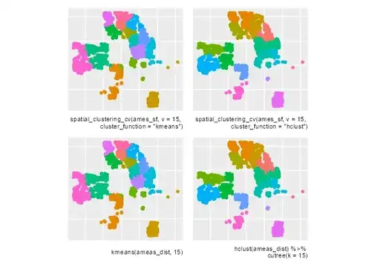
Visual comparison of different methods:

list(
  ggplot(clust_fkm) +
    labs(caption = 'spatial_clustering_cv(ames_sf, v = 15, \ncluster_function = "kmeans")') +
    geom_sf(aes(color = id)),
  ggplot(clust_fhcl) +
    labs(caption = 'spatial_clustering_cv(ames_sf, v = 15, \ncluster_function = "hclust")') +
    geom_sf(aes(color = id)),
  ggplot(ames_sf) +
    labs(caption = 'kmeans(ameas_dist, 15)') +
    geom_sf(aes(color = kmeans_clust)),
  ggplot(ames_sf) +
    labs(caption = 'hclust(ameas_dist) %>% \ncutree(k = 15)') +
    geom_sf(aes(color = hclust))
) %>% 
  map(~ .x + theme(legend.position = "none", 
                   axis.text = element_blank(),
                   axis.ticks = element_blank())) %>% 
  patchwork::wrap_plots()

^{Created on 2023-07-12 with reprex v2.0.2}