Get X of Very Large Polynomial at Y? (Python 3.10, NumPy)

Question

I'm attempting to calculate all real X-values, at a certain Y-value, of a 20-degree polynomial provided in a coefficent list of ascending powers. I'm using Python 3.10 as well as the roots function of the NumPy library.

(I previously posted a simillar question here on StackOverflow, attempting to solve this issue by producing a much simpler example with a far smaller polynomial. However, while the solution to that posting did solve the issue for small polynomials, it did not solve the issue for when I use large polynomials.)

Here is my example code:

import numpy as np
import matplotlib.pyplot as plt

def main():
    # Declare 20-degree polynomial
    coeffs = np.array([0.028582380269090664, -11.07209382330515, 81.98886137780704, -231.55726577581814, 344.8963540923082, -312.0774305574022, 185.36300988588312, -75.58767327080196, 21.660357329823697, -4.380346453954649, 0.6125779086029393, -0.05524029639869697, 0.002489646479713822, 4.159253423505381e-05, -9.927184104751197e-06, 8.634292922740336e-08, 3.278890552085848e-08, -3.350925351280405e-10, -1.1510786631391544e-10, -2.3053456641329463e-13, 3.9927010006271344e-13, 8.499990550259627e-15, -1.2514130885401332e-15, -5.653183054629818e-17, 3.5580325101956145e-18, 2.634844330077943e-19, -1.2086461102288157e-20, -9.772155900613053e-22, 8.336597931160041e-23, -2.286862805703104e-24, 2.2638043801338818e-26], dtype = float)
    y = -5

    # Create polynomial data on interval (0, 17)
    polyDataX = np.linspace(0, 17)
    polyDataY = np.empty(shape = len(polyDataX), dtype = float)

    for i in range(len(polyDataX)):
        polyDataY[i] = 0

        for j in range(len(coeffs)):
            polyDataY[i] += coeffs[j] * pow(polyDataX[i], j)

    # Solve for all real solutions
    coeffs[-1] -= y
    sols = np.roots(coeffs).tolist()
    i = 0

    while (i < len(sols)):
        if (sols[i].imag != 0) or (sols[i].real < 0) or (sols[i].real > 17):
            del sols[i]
            i -= 1
        else:
            sols[i] = round(sols[i].real, 2)

        i += 1

    # Plot polynomial & solutions
    plt.xlim([0, 17])
    plt.ylim([-30, 30])
    plt.plot(polyDataX, polyDataY, color = "gray")
    plt.axhline(y, color = "blue")
    
    for sol in sols:
        plt.axvline(sol, color = "red")

    plt.title("Sols: " + str(sols))
    plt.show()
    plt.close()
    plt.clf()

if (__name__ == "__main__"):
    main()

First I generate a 20-degree polynomial (stored in coeffs), and use the roots function in order to acquire all X-values (stored in sols), at a certain Y-value (stored in y). I subsequently filter out all the imaginary solutions, leaving only the real ones at the desired interval of [0, 17], and I plot the plolynomial, alongside the desired Y-value and found real X-values. I colored the polynomial in gray, the desired Y-value in blue and all the filtered X-values in red.

In the above example, I attempt to acquire all real X-values at a the Y-value of -5. The X-values are listed as [3.92, 1.34, 1.13], which is clearly incorrect according to the generated plot:

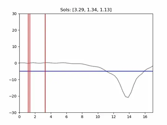
According to the plot, the actual X-values for a Y-value of -5 should be ~11.2 and ~16.

What am I doing wrong here? Why are the listed solutions from the roots function incorrect here?

Thanks for reading my post, any guidance is appreciated.

You said you're using a 20-degree polynomial, but `coeffs` is of length 31. — jared, Jul 03 '23 at 21:52
I just added a new answer to your original question that makes use of the `np.polynomial.Polynomial` class. Using that method will make your code much simpler and might solve this issue. — jared, Jul 03 '23 at 22:11
why not use `sols = [ round(s.real, 2) for s in sols if s.imag == 0.0 and (0.0 < s.real < 17.0)]` — rioV8, Jul 03 '23 at 23:20

Reinderien · Accepted Answer · 2023-07-04T00:55:26.350

2

Delete most of your code and use the built-in Polynomial support:

import numpy as np
import matplotlib.pyplot as plt
from numpy.polynomial import Polynomial


def get_roots(poly: Polynomial, y: float = 0) -> np.ndarray:
    roots = (poly - y).roots()
    real_roots = roots.real[np.isreal(roots)]
    return real_roots[
        (poly.domain[0] <= real_roots) &
        (poly.domain[1] >= real_roots)
    ]


def plot(poly: Polynomial, real_roots: np.ndarray, y: float) -> plt.Figure:
    x = np.linspace(6, poly.domain[1], num=1_000)

    fig, ax = plt.subplots()
    ax.set_title(f"Roots of degree-{poly.degree()} polynomial")
    ax.set_ylim(-1, 1)
    ax.axhline(y, c='black', linewidth=0.5)
    ax.plot(x, poly(x))
    for root in real_roots:
        ax.annotate(
            text=f'{root:.3f}',
            xy=(root, y),
            xytext=(root - 0.5, -0.6),
            arrowprops={'arrowstyle': '-'},
        )

    return fig


def main() -> None:
    coeffs = np.array([
        2.85823803e-02, -1.10720938e+01,  8.19888614e+01, -2.31557266e+02,
        3.44896354e+02, -3.12077431e+02,  1.85363010e+02, -7.55876733e+01,
        2.16603573e+01, -4.38034645e+00,  6.12577909e-01, -5.52402964e-02,
        2.48964648e-03,  4.15925342e-05, -9.92718410e-06,  8.63429292e-08,
        3.27889055e-08, -3.35092535e-10, -1.15107866e-10, -2.30534566e-13,
        3.99270100e-13,  8.49999055e-15, -1.25141309e-15, -5.65318305e-17,
        3.55803251e-18,  2.63484433e-19, -1.20864611e-20, -9.77215590e-22,
        8.33659793e-23, -2.28686281e-24,  2.26380438e-26])
    y = -0.1
    poly = Polynomial(coeffs, domain=(0, 17))
    real_roots = get_roots(poly, y)
    plot(poly, real_roots, y)
    plt.show()


if __name__ == "__main__":
    main()

edited Jul 04 '23 at 00:55

answered Jul 04 '23 at 00:10

Reinderien

11,755
5
49
77

This is what I said on their last question. Though, you have to be careful because `Polynomial` expects the coefficients ordered from lowest to highest order. Based on their last question, they probably shared the coefficients in reverse. – jared Jul 04 '23 at 00:15
1

@jared Whether they accidentally reversed the order of the coefficient array or not, observe `coeffs[j] * pow(polyDataX[i], j)` - they already assume lowest to highest. – Reinderien Jul 04 '23 at 00:16
Further, reversing the coefficients produces a true mess of roots that does not look like their original graph. – Reinderien Jul 04 '23 at 00:18
1

Ah, yes, you're right. They're creating their polynomial differently this time. And I didn't run the code to see which order made sense, so I'll take your word on that. – jared Jul 04 '23 at 00:19
Also, OP wants the solutions for a specific `y` value, not just `y=0`. So, you can probably add an option `y` argument (defaulting to 0) and can evaluate the roots as I showed on my solution for their original question, i.e. `roots = (poly - y).roots()`. – jared Jul 04 '23 at 00:24
@jared true; this should be better (though the original -5 does not produce any roots) – Reinderien Jul 04 '23 at 00:43
Is there a reason it's better to change the coefficient rather than create the `Polynomial` object and pass that to the `get_roots` function where you can do what I mentioned above to get the desired roots? – jared Jul 04 '23 at 00:48
Passing the polynomial and evaluating the roots how I mentioned shouldn't be in-place, so you wouldn't effect the polynomial object. – jared Jul 04 '23 at 00:50
Seems like six of one, half a dozen of the other? Either you change the coefficients out-of-place, or you change the polynomial out-of-place. – Reinderien Jul 04 '23 at 00:50
To me, it seems cleaner because it has less repeated code and makes use of the same `Polynomial` object you already created and are passing to the plotting function. – jared Jul 04 '23 at 01:00

Get X of Very Large Polynomial at Y? (Python 3.10, NumPy)

1 Answers1