The best approach to preventing the value of the Kullback–Leibler divergence becoming infinite

Question

Given two discrete probability distributions P and Q, containing zero values in some bins, what is the best approach to avoid the Kullback–Leibler divergence equal to infinite (and therefore getting some finite value, between zero and one)?

Here below an example of calculation (with Matlab) of the Kullback–Leibler divergence between P and Q, which gives an infinite value. I am tempted to manually remove "NaNs" and "Infs" from "log2( P./Q )", but I am afraid this is not correct. In addition, I am not sure that smoothing the PDFs could solve the issue...

% Input
A =[     0.444643925792938         0.258402203856749
         0.224416517055655         0.309641873278237
        0.0730101735487732         0.148209366391185
        0.0825852782764812        0.0848484848484849
        0.0867743865948534        0.0727272727272727
        0.0550568521843208        0.0440771349862259
       0.00718132854578097        0.0121212121212121
       0.00418910831837223        0.0336088154269972
       0.00478755236385398        0.0269972451790634
       0.00359066427289048       0.00110192837465565
       0.00538599640933573       0.00220385674931129
      0.000598444045481747                         0
       0.00299222022740874       0.00165289256198347
                         0                         0
       0.00119688809096349      0.000550964187327824
                         0      0.000550964187327824
       0.00119688809096349      0.000550964187327824
                         0      0.000550964187327824
                         0      0.000550964187327824
      0.000598444045481747                         0
      0.000598444045481747                         0
                         0                         0
                         0      0.000550964187327824
                         0                         0
                         0                         0
                         0                         0
                         0                         0
                         0                         0
                         0                         0
                         0                         0
                         0                         0
                         0                         0
                         0                         0
                         0                         0
                         0                         0
                         0                         0
                         0      0.000550964187327824
                         0                         0
                         0                         0
                         0                         0
                         0                         0
                         0                         0
                         0                         0
                         0                         0
                         0                         0
                         0                         0
                         0                         0
                         0                         0
                         0                         0
       0.00119688809096349      0.000550964187327824];
P   = A(:,1); % sum(P) = 0.999999999
Q   = A(:,2); % sum(Q) = 1

% Calculation of the Kullback–Leibler divergence
M   = numel(P);                   
P   = reshape(P,[M,1]);           
Q   = reshape(Q,[M,1]);
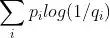
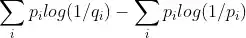
KLD = nansum( P .* log2( P./Q ) )

% Result
>> KLD

KLD =

   Inf

>> log2( P./Q )

ans =

         0.783032102845145
         -0.46442172001576
         -1.02146721017182
       -0.0390042690948072
         0.254772785478407
         0.320891675991577
        -0.755211303094213
         -3.00412460068336
         -2.49545202929328
          1.70422031554308
          1.28918281626424
                       Inf
         0.856223408988134
                       NaN
          1.11925781482192
                      -Inf
          1.11925781482192
                      -Inf
                      -Inf
                       Inf
                       Inf
                       NaN
                      -Inf
                       NaN
                       NaN
                       NaN
                       NaN
                       NaN
                       NaN
                       NaN
                       NaN
                       NaN
                       NaN
                       NaN
                       NaN
                       NaN
                      -Inf
                       NaN
                       NaN
                       NaN
                       NaN
                       NaN
                       NaN
                       NaN
                       NaN
                       NaN
                       NaN
                       NaN
                       NaN
          1.11925781482192

FIRST EDITING

So far, I found a theoretical argument, which partially solve my issue, but still, the infinite values remain when

% if P_i > 0 and Q_i = 0, then P_i*log(P_i/0) = Inf

The following is what I implemented by considering the conventions described at pag.19 of "Elements of Information Theory, 2nd Edition Thomas M. Cover, Joy A. Thomas":

clear all; close all; clc;
% Input
A =[     0.444643925792938         0.258402203856749
         0.224416517055655         0.309641873278237
        0.0730101735487732         0.148209366391185
        0.0825852782764812        0.0848484848484849
        0.0867743865948534        0.0727272727272727
        0.0550568521843208        0.0440771349862259
       0.00718132854578097        0.0121212121212121
       0.00418910831837223        0.0336088154269972
       0.00478755236385398        0.0269972451790634
       0.00359066427289048       0.00110192837465565
       0.00538599640933573       0.00220385674931129
      0.000598444045481747                         0
       0.00299222022740874       0.00165289256198347
                         0                         0
       0.00119688809096349      0.000550964187327824
                         0      0.000550964187327824
       0.00119688809096349      0.000550964187327824
                         0      0.000550964187327824
                         0      0.000550964187327824
      0.000598444045481747                         0
      0.000598444045481747                         0
                         0                         0
                         0      0.000550964187327824
                         0                         0
                         0                         0
                         0                         0
                         0                         0
                         0                         0
                         0                         0
                         0                         0
                         0                         0
                         0                         0
                         0                         0
                         0                         0
                         0                         0
                         0                         0
                         0      0.000550964187327824
                         0                         0
                         0                         0
                         0                         0
                         0                         0
                         0                         0
                         0                         0
                         0                         0
                         0                         0
                         0                         0
                         0                         0
                         0                         0
                         0                         0
       0.00119688809096349      0.000550964187327824];
P   = A(:,1);
Q   = A(:,2);
% some processing
M   = numel(P);                   
P   = reshape(P,[M,1]);           
Q   = reshape(Q,[M,1]);

% At Pag.19 of "Elements of Information Theory, 2nd Edition Thomas M. Cover, Joy A. Thomas"
% (Section: 2.3 Relative Entropy and Mutual Information)
% there are three conventions to be used in the calculation of the Kullback–Leibler divergence
idx1 = find(P==0 & Q>0);  % index for convention 0*log(0/q) = 0
idx2 = find(P==0 & Q==0); % index for convention 0*log(0/0) = 0
idx3 = find(P>0 & Q==0);  % index for convention p*log(p/0) = Inf

% Calculation of the Kullback–Leibler divergence, 
% by applying the three conventions described in "Elements of Information Theory..."
tmp = P .* log2( P./Q );
tmp(idx1) = 0;            % convention 0*log(0/q) = 0
tmp(idx2) = 0;            % convention 0*log(0/0) = 0
tmp(idx3) = Inf;          % convention p*log(p/0) = Inf
KLD = sum(tmp)

The result is still "Inf" since some elements in the distribution Q are zeros, while the corresponding elements of P are greater than zero:

KLD =

   Inf

SECOND EDITING, i.e. after the first @Meferne Answer (PLEASE, DO NOT USE THIS CODE - IT LOOKS LIKE I MISUNDERSTOOD THE @Meferne COMMENT)

I tried to apply the softmax function to the distribution Q (in order to have Q_i>0), but the distribution Q changes considerably:

P   = A(:,1);
Q   = A(:,2);
% some processing
M   = numel(P);                   
P   = reshape(P,[M,1]);           
Q   = reshape(Q,[M,1]);

Q   = softmax(Q); % <-- this is equivalent to: Q = softmax(Q) = exp(Q)/sum(exp(Q))

% At Pag.19 of "Elements of Information Theory, 2nd Edition Thomas M. Cover, Joy A. Thomas"
% (Section: 2.3 Relative Entropy and Mutual Information)
% there are three conventions to be used in the calculation of the Kullback–Leibler divergence
idx1 = find(P==0 & Q>0);  % index for convention 0*log(0/q) = 0
idx2 = find(P==0 & Q==0); % index for convention 0*log(0/0) = 0
idx3 = find(P>0 & Q==0);  % index for convention p*log(p/0) = Inf

% Calculation of the Kullback–Leibler divergence, 
% by applying the three conventions described in "Elements of Information Theory..."
tmp = P .* log2( P./Q );
tmp(idx1) = 0;            % convention 0*log(0/q) = 0
tmp(idx2) = 0;            % convention 0*log(0/0) = 0
tmp(idx3) = Inf;          % convention p*log(p/0) = Inf
KLD = sum(tmp)

...leading to a KLD value greater than 1:

KLD =

       2.9878

THIRD EDITING, i.e. after further explanatory comments of @Meferne (PLEASE USE THIS CODE IF NEEDED!)

clear all; close all; clc;
format long G % <-- to see better that the "sum(Qtmp)" is greater than 1
% Input
A =[     0.444643925792938         0.258402203856749
         0.224416517055655         0.309641873278237
        0.0730101735487732         0.148209366391185
        0.0825852782764812        0.0848484848484849
        0.0867743865948534        0.0727272727272727
        0.0550568521843208        0.0440771349862259
       0.00718132854578097        0.0121212121212121
       0.00418910831837223        0.0336088154269972
       0.00478755236385398        0.0269972451790634
       0.00359066427289048       0.00110192837465565
       0.00538599640933573       0.00220385674931129
      0.000598444045481747                         0
       0.00299222022740874       0.00165289256198347
                         0                         0
       0.00119688809096349      0.000550964187327824
                         0      0.000550964187327824
       0.00119688809096349      0.000550964187327824
                         0      0.000550964187327824
                         0      0.000550964187327824
      0.000598444045481747                         0
      0.000598444045481747                         0
                         0                         0
                         0      0.000550964187327824
                         0                         0
                         0                         0
                         0                         0
                         0                         0
                         0                         0
                         0                         0
                         0                         0
                         0                         0
                         0                         0
                         0                         0
                         0                         0
                         0                         0
                         0                         0
                         0      0.000550964187327824
                         0                         0
                         0                         0
                         0                         0
                         0                         0
                         0                         0
                         0                         0
                         0                         0
                         0                         0
                         0                         0
                         0                         0
                         0                         0
                         0                         0
       0.00119688809096349      0.000550964187327824];
P   = A(:,1);
Q   = A(:,2);
% some processing
M   = numel(P);                   
P   = reshape(P,[M,1]);           
Q   = reshape(Q,[M,1]);

% renormalize the distribution Q (after the comments of @Meferne)
epsilon = 1e-12;
Qtmp = Q;               % <-- assign temporarily the distribution Q to another array
Q = [];                 % <-- delete/empty Q
Qtmp = Qtmp + epsilon;  % <-- add a small positive number (epsilon) to all Q_i
sum(Qtmp)               % <-- just to check: the sum of all Q_i is now greater than 1 (as expected)
Q = Qtmp./sum(Qtmp);    % <-- renormalize the distribution Q
sum(Q)                  % <-- just to check: the sum of all Q_i is again equal to 1 (as expected)

% At Pag.19 of "Elements of Information Theory, 2nd Edition Thomas M. Cover, Joy A. Thomas"
% (Section: 2.3 Relative Entropy and Mutual Information)
% there are three conventions to be used in the calculation of the Kullback–Leibler divergence
idx1 = find(P==0 & Q>0);  % index for convention 0*log(0/q) = 0
idx2 = find(P==0 & Q==0); % index for convention 0*log(0/0) = 0
idx3 = find(P>0 & Q==0);  % index for convention p*log(p/0) = Inf

% Calculation of the Kullback–Leibler divergence, 
% by applying the three conventions described in "Elements of Information Theory..."
tmp = P .* log2( P./Q );
tmp(idx1) = 0;            % convention 0*log(0/q) = 0
tmp(idx2) = 0;            % convention 0*log(0/0) = 0
tmp(idx3) = Inf;          % convention p*log(p/0) = Inf
KLD = sum(tmp)

Which leads to:

sum(Qtmp) =
             1.00000000005
sum(Q)    =
                         1
KLD       =
         0.247957353229104

Use Krichevsky-Trofimov correction https://en.wikipedia.org/wiki/Krichevsky%E2%80%93Trofimov_estimator — Severin Pappadeux, Jun 29 '23 at 19:25
HEre is nice summary https://nemenmanlab.org/~ilya/images/e/e2/NIPS-01-poster.pdf — Severin Pappadeux, Jun 29 '23 at 19:32

score 1 · Accepted Answer · answered Jun 29 '23 at 04:12

1

Let's say you were doing machine learning, and P was the ground truth probability distribution, and Q was the predicted distribution.

The goal would be to minimize the KL divergence between P and Q (in practice, the related cross-entropy, which has the same minimum point as KL).

Now, the edge case that worries you is the one where the ground truth value is different than 0, while the predicted value is zero. This is the case that would have infinite KL divergence (or infinite loss in machine learning). As you've put it, that's the case where P_i > 0and Q_i = 0.

The bottom line is that conceptually, it does make sense to define such cases to have +inf KL divergence. That would be the maximum (infinite) loss while doing machine learning and cross-entropy loss minimization.

In practice, the question is what's your underlying reason to do this calculation in the first place.

In machine learning, you would be minimizing just the cross-entropy term

equation using Online Equation Editor

while you have the full KL

equation using Online Equation Editor

The issue for you here is the log q_i part which diverges to -infat zero.

In machine learning, it would often be the softmax activation function that produces all q_i, ensuring that they would all end up strictly positive. In addition, it is typically the logsoftmax function that does both the log and softmax calculation together, rather than first calculating q_i and then doing the log. This approach is numerically more stable.

So, if this is relevant to your case, possibly you could go back and redefine all q_i to become strictly positive. And if there is a softmax calculation that produces all q_i, you can also join it with log. You can refer to this logsoftmax implementation in numpy: https://stackoverflow.com/a/61570752/5235274

As an alternative, another approach that might be relevant for you is to use Jensen-Shannon divergence instead of KL:

Since you're using this to build the Jensen-Shannon divergence the only way that you can have qi equal to zero in the calculation of the Kullback-Leibler divergence is if the pi value is also zero. This is because really you're calculating the average of dKL(p,m) and dKL(q,m), where m=(p+q)/2. So mi=0 implies both pi=0 and qi=0.

https://stackoverflow.com/a/10003064/5235274

If you switch to Jensen-Shannon instead of KL, you will avoid this problem where the second distribution has zero values while the first one doesn't. In addition, this one is bounded between 0 and 1, which you also stated as a desired goal. KL divergence is not bounded.

It is based on the Kullback–Leibler divergence, with some notable (and useful) differences, including that it is symmetric and it always has a finite value.

https://en.wikipedia.org/wiki/Jensen%E2%80%93Shannon_divergence

answered Jun 29 '23 at 04:12

meferne

349
2
9

Thanks a lot @meferne!! I have tried the path of the "softmax", which you can find in my original post after the section ```SECOND EDITING, i.e. after the @Meferne Answer```....However, I am not sure about it...... :-) :-) – limone Jun 29 '23 at 11:22
1

@limone, oh, softmax is not for your current `q_i` distribution directly. It's only relevant if you can pose your problem so that you have some starting vector of the same size `z` as `q`, and then define `q = softmax(z)`. It would help to know more about the problem you are solving. A simple solution for you might be to add some small epsilon to all q, and to renormalize all to sum to 1. That's also an important point: your P and Q should be normalized to sum to 1. Probably the best option for you is Jensen-Shannon. Note that KL is generally not bound to be less than 1, while JS is. – meferne Jun 29 '23 at 13:00
thanks @mefreme... I might have misunderstood your answer... basically I have two histograms (then converted into two discrete probability distributions, which sum of probabilities is 1, for both distributions) that I need to compare... About the solution "to add a small epsilon to all q, and then to renormalize all", what formula would you mean by "renormalize all to sum to 1"? (so that, I can try).....and, yes, I can use the Jensen-Shannon div as well.. but I would like to use the KLD as well, if possible.. – limone Jun 29 '23 at 13:50
1

@limone, you add a small positive number (epsilon) to all `q_i`. Note that when you do that, the sum of all `q_i` will become larger than 1. You take that sum, and divide all current `q_i` values by that value. The final values will all be positive, and their sum will be 1 again. From what you said so far, since you want bounded final values, and you probably also want the comparison between P and Q to be symmetric, I'd go with JS. KL is not symmetric, and you will still get high final values with the epsilon approach. – meferne Jun 29 '23 at 14:44
1

Many thanks @meferne!!! It now works..! Please see what I wrote after the```THIRD EDITING, i.e. after further explanatory comments of @Meferne``` in my original post.. I might have a last question or doubt....is there any theoretical argument for this trick (i.e. add an epsilon in Q and then re-normalise the same distribution Q)? Could it be a trick similar to what used in ```R``` and called as the "Laplace correction"? (Please see another - possibly related question - at https://stats.stackexchange.com/questions/620077/laplace-correction-in-r?noredirect=1#comment1153244_620077 ) – limone Jun 29 '23 at 15:10
Yes, I will now pass to implement the Jensen-Shannon div... thanks :-) – limone Jun 29 '23 at 15:11
1

@limone You are welcome! :) The epsilon approach is common when there is possible division by zero or log zero calculation. The re-normalization is to still have the probability distribution properties, i.e., summing to 1. But it turns out that this technique in this context does have a special name: Additive or Laplace smoothing. https://www.wikiwand.com/en/Additive_smoothing It's the same thing, but applied to raw histogram counts, before any normalization. Note how they add a fixed number to each histogram bin, and then they divide by the new sum for normalization. – meferne Jun 29 '23 at 16:00
1

Also, the larger the number you add, the starting distribution becomes more smooth. You can justify this as adding some starting prior knowledge to the actual measurements, which are always inexact. – meferne Jun 29 '23 at 16:04
1

Great Answer @meferne! It is a relief to know that this technique has an historical reference (i.e. the "Additive or Laplace smoothing")... Many thanks :-) :-) – limone Jun 29 '23 at 16:13
@maferne...I have two tiny doubts........(FIRST DOUBT) by applying the re-normalization (i.e. what I did within the```THIRD EDITING, i.e. after further explanatory comments of @Meferne```), will the KLD be still unbounded, i.e. ```0<=KLD – limone Jun 30 '23 at 08:22
(SECOND DOUBT) Should the re-normalization be applied directly to the distribution Q, as I did within the ```THIRD EDITING, i.e. after...```? I got this doubt when I looked into https://www.wikiwand.com/en/Additive_smoothing. Indeed, I tried to find the similarities between what I did in ```THIRD EDITING,...``` and the estimator,```$\theta_i = \frac{x_i+\alpha}{N+\alpha d}$```. I would say that the set of observations ```$\lt x_1,x_2,...,x_d\gt$``` would correspond to my ```Q_i```, while the re-normalised values of Q, would correspond to ```\theta_i```. Is it correct? – limone Jun 30 '23 at 08:36
@maferne, obviously, if my two doubts are already considered as "full questions" in stackoverflow, I can open another thread.. – limone Jun 30 '23 at 08:45
1

@limone 1. KL is still unbounded. Check my previous comments why I suggested Jensen Shannon instead. 2. In the additive smoothing approach, all x_1, x_2, ... x_n sum to N. Those are raw counts, while your starting q_i already sum to 1. You can just keep it as is with the epsilon, or you can go back to the original histogram values before you computed your initial q_i to apply the additive smoothing like in that link. Note though that if you set N=1 and assume x_i sum to 1, that formula exactly gives what you are doing now with the epsilon. – meferne Jun 30 '23 at 09:40

The best approach to preventing the value of the Kullback–Leibler divergence becoming infinite

1 Answers1