Display calculated value per facet per frame using gganimate

Question

I am trying to summarize the Pearson correlation index between x and y per facet (grouping) z and per frame by transition_filter

data.frame(x = runif(300), y = runif(300), z = runif(300), g = rep(c("a", "b", "c"), each = 100)) %>%
  ggplot(aes(x = x, y = y, color = z)) + geom_point() +
  facet_wrap(. ~ g) +
  transition_filter(transition_length = 1, filter_length = 1,
                    z >= 0.5 & z < 0.6,
                    z >= 0.6 & z < 0.7,
                    z >= 0.7 & z < 0.8,
                    z >= 0.8 & z < 0.9,
                    z >= 0.9 & z < 1) +
  geom_text(aes(label = paste0("Cor = ", cor(x, y))), x = 0.25, y = 1) +
  ggtitle('{closest_expression}')

I can get the correlation indexes displayed though they appear to be the same across facets and frames:

What is the correct way of doing this?

The image is placed in a wrong position, but I am not allowed to edit my post, there is always an error prompt — Tianjian Qin, Jun 16 '23 at 16:24

Jon Spring · Accepted Answer · 2023-06-16T18:43:09.250

This sounds like an ambitious case for gganimate, which I don't think is currently set up to do by-facet calculations per frame. (Curious to see if anyone else knows a way.) My go-to approach for showing unusual things with gganimate is to calculate what we want to show before sending to ggplot2.

df1 <- data.frame(x = runif(300), y = runif(300), z = runif(300), 
                  g = rep(c("a", "b", "c"), each = 100)) |>
  mutate(case = case_when(
    z < 0.5 ~ NA,
    .default = cut(z, seq(0.5, 1, 0.1))
  ))

df1_cor <- df1  |>
  summarise(cor = cor(x, y), .by = c(case, g))

df1 |>
  ggplot(aes(x = x, y = y)) + 
  geom_point(aes(color = z)) +
  facet_wrap(. ~ g) +
  transition_manual(case) +
  geom_text(aes(label = scales::number(cor, accuracy = 0.0001)),
            x = 0.25, y = 1, data = df1_cor) +
  ggtitle('{current_frame}')

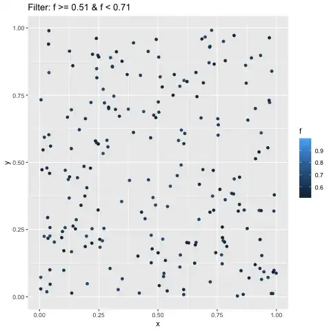
Per the OP comment about to deal with overlapping cases, we could use a similar approach. We can construct our cases, join the data to match all the observations that go with each case, and plot that.

df <- data.frame(x = runif(1000), y = runif(1000), f = runif(1000))
df2 <- data.frame(low = seq(0.51, 0.8, 0.01), high = seq(0.71, 1, 0.01)) |>
  mutate(nice_name = paste0("Filter: f >= ", low, " & f < ", high)) |>
  left_join(df, join_by(low <= f, high > f))

df2 |>
  ggplot(aes(x = x, y = y)) + 
  geom_point(aes(color = f)) +
  transition_manual(nice_name) +
  ggtitle('{current_frame}')

Could you please elaborate more about if, say I have a large number of cases, as I described in https://stackoverflow.com/questions/76489657/filter-data-frame-by-multiple-conditions-stored-in-one-string-using-gganimate, how to use the filering conditions stored in a vector? Much appreciated. — Tianjian Qin, Jun 16 '23 at 17:01
See edit. We can construct our cases, join the data to match all the observations that go with each case, and plot that. — Jon Spring, Jun 16 '23 at 17:46

score 1 · Answer 2 · answered Jun 16 '23 at 17:29

Here is a solution with more animation. But for me it was not possible to remove the stop sequences!

library(gganimate)
library(tidyverse)

# z-range
df$z_range <- cut(df$z, breaks = seq(0.5, 1, by = 0.1))

# Corrleation by group
correlations <- df %>%
  group_by(g, z_range) %>%
  summarise(correlation = cor(x, y, use = "pairwise.complete.obs"), .groups = "drop")

# plot
left_join(df, correlations, by = c("g", "z_range")) %>% 
  ggplot(aes(x = x, y = y, color = z)) + 
  geom_point() +
  facet_wrap(. ~ g) +
  transition_states(z_range, transition_length = 1, state_length = 1) +
  enter_fade() + 
  exit_fade() +
  geom_text(data = correlations, 
            aes(label = paste0("Cor = ", round(correlation, 2)), 
                x = 0.5, 
                y = 1), 
            size = 5, 
            check_overlap = TRUE, 
            inherit.aes = FALSE) +
  labs(title = 'Transition {closest_state}')

Display calculated value per facet per frame using gganimate

2 Answers2