Combining multiple datasets in one scatterplot with R

Question

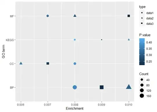
I have three datasets which I would like combine in one scatter plot. The data sets are: data 1 -

GO term	Count	Enrichment	P value
BP	163	0.008	0.37
MF	48	0.007	0.33
CC	58	0.008	0.39
KEGG	27	0.008	0.43

data 2 -

GO term	Count	Enrichment	P value
BP	167	0.01	0.31
MF	50	0.008	0.29
CC	50	0.006	0.34
KEGG	23	0.01	0.37

data 3 -

GO term	Count	Enrichment	P value
BP	123	0.009	0.22
MF	44	0.01	0.22
CC	50	0.007	0.24
KEGG	14	0.009	0.28

## to reproduce
data_1 <- structure(list(GO.term = c("BP", "MF", "CC", "KEGG"), Count = c(163L, 
48L, 58L, 27L), Enrichment = c(0.008, 0.007, 0.008, 0.008), P.value = c(0.37, 
0.33, 0.39, 0.43)), class = "data.frame", row.names = c(NA, 4L
))

data_2 <- structure(list(GO.term = c("BP", "MF", "CC", "KEGG"), Count = c(167L, 
50L, 50L, 23L), Enrichment = c(0.01, 0.008, 0.006, 0.01), P.value = c(0.31, 
0.29, 0.34, 0.37)), class = "data.frame", row.names = c(NA, 4L
))

data_3 <- structure(list(GO.term = c("BP", "MF", "CC", "KEGG"), Count = c(123L, 
44L, 50L, 14L), Enrichment = c(0.009, 0.01, 0.007, 0.009), P.value = c(0.22, 
0.22, 0.24, 0.28)), class = "data.frame", row.names = c(NA, 4L
))

For data 1, I created a scatterplot with ggplot(data, aes(x=Fold.Enrichment, y=GO.Term, color=PValue)) + geom_point(aes(size=Count))

Now I want to combine all the data sets in one plot. Is it possible with scatterplot or do I need to change the graph type?

`bind_rows()` will combine the three datasets into one. Whether that's sufficient for your pruposes will depend on exactly what you want th scatter plot to show. Note that your sample code is not consistent with your sample data: the column names are different. — Limey, Jun 16 '23 at 12:24

score 1 · Answer 1 · edited Jun 17 '23 at 12:51

Here is a way to use bind_rows to combine all the datasets. Notice that I'm using mutate to add a type column in order for you to differentiate between them, here using different shape for each type.

library(tidyverse)

data_1 <-
  structure(
    list(
      GO.term = c("BP", "MF", "CC", "KEGG"),
      Count = c(163L,
                48L, 58L, 27L),
      Enrichment = c(0.008, 0.007, 0.008, 0.008),
      P.value = c(0.37,
                  0.33, 0.39, 0.43)
    ),
    class = "data.frame",
    row.names = c(NA, 4L)
  )

data_2 <-
  structure(
    list(
      GO.term = c("BP", "MF", "CC", "KEGG"),
      Count = c(167L,
                50L, 50L, 23L),
      Enrichment = c(0.01, 0.008, 0.006, 0.01),
      P.value = c(0.31,
                  0.29, 0.34, 0.37)
    ),
    class = "data.frame",
    row.names = c(NA, 4L)
  )

data_3 <-
  structure(
    list(
      GO.term = c("BP", "MF", "CC", "KEGG"),
      Count = c(123L,
                44L, 50L, 14L),
      Enrichment = c(0.009, 0.01, 0.007, 0.009),
      P.value = c(0.22,
                  0.22, 0.24, 0.28)
    ),
    class = "data.frame",
    row.names = c(NA, 4L)
  )

bind_rows('data1' = data_1,
  'data2' = data_2,
  'data3' = data_3,
  .id = 'type') %>%
  ggplot(aes(
    x = Enrichment,
    y = GO.term,
    col = P.value,
    size = Count,
    shape = type
  )) +
  geom_point()

^{Created on 2023-06-16 with reprex v2.0.2}

You can also do this with a single use of `bind_rows`: `bind_rows('data1' = data_1, 'data2' = data_2, 'data3' = data_3, .id = 'type')` — Seth, Jun 16 '23 at 13:14
That is much cleaner, feel free to edit the answer accordingly! — mhovd, Jun 16 '23 at 13:33

I_O · Accepted Answer · 2023-06-16T13:43:12.490

an alternative is to facet your plot (one panel per data source):

combine dataframes to one, adding a source column:

data_combined <- 
  paste0('data_', 1:3) |> ## the names of your single dataframes
  Map(f = \(source) cbind(source, get(source))) |>
  Reduce(f = rbind)

plot and facet with ggplot:

library(ggplot2)

data_combined |>
  ggplot() +
  geom_point(aes(Enrichment,
                 GO.term,
                 size = Count,
                 color = P.value,
                 )
             ) +
  facet_wrap(~ source, ncol = 1)

aside: benchmark rbind vs bind_rows

## binds dataframes data_1:data_3 by row, using bind_function:
bind_them <- \(bind_function){
  combined <- 
    paste0('data_', 1:3) |> 
    Map(f = \(source) cbind(source, get(source))) |>
    Reduce(f = bind_function)
}


microbenchmark::microbenchmark(bind_them('rbind'), bind_them('bind_rows'),
                               control = list(warmup = 2 ))

Unit: microseconds
                   expr    min      lq     mean  median     uq    max neval cld
     bind_them("rbind")  805.1  827.75  968.666  925.55  955.7 2145.6   100  a 
 bind_them("bind_rows") 3721.6 3795.35 4251.423 4061.25 4349.8 9032.2   100   b

Note that `rbind` is _much_ slower than `bind_rows`, and have a few key differences (https://stackoverflow.com/a/59482527/3212698). — mhovd, Jun 16 '23 at 13:06
I was surprised that `dplyr` should be more convenient **and** faster than the corresponding base-R function, so I run a `microbenchmark`. As expected, `rbind` did the job in a quart of the time, at least in the use case at hand (see edit please). — I_O, Jun 16 '23 at 13:46

Combining multiple datasets in one scatterplot with R

2 Answers2