How to bold/thicken state border on maps made in R while including county borders?

Question

I am trying to map all 50 US states and their respective counties. But I specifically want to thicken/bold the US state borders while keeping the county borders thin.

This is the code I have tried to map my data. Please note that I had to use a different code to modify the locations of Alaska and Hawaii.

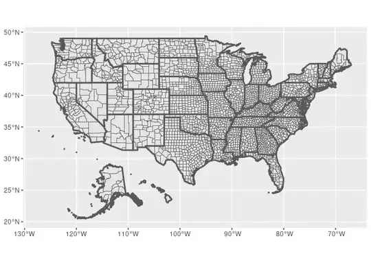
First this is the code to map county borders and the resulting map.

map_sf <- tigris::counties(cb = T, class = 'sf')
# removed US territories
map_sf <- map_sf %>% filter(!STATEFP %in% c('60', '66', '69', '72', '78'))
# CRS code to modify Alaska and Hawaii location
crs_lambert <- "+proj=laea +lat_0=45 +lon_0=-100 +x_0=0 +y_0=0 +a=6370997 +b=6370997 +units=m +no_defs"
map_sf <- map_sf %>%
  st_transform(crs = crs_lambert)
alaska <- map_sf %>% filter(STATE_NAME %in% 'Alaska')
alaska_g <- st_geometry(alaska)
alaska_centroid <- st_centroid(st_union(alaska_g))
rot <- function(a) matrix(c(cos(a), sin(a), -sin(a), cos(a)), 2, 2)
alaska_trans <- (alaska_g - alaska_centroid) * rot(-39 * pi/180) / 2.3 + alaska_centroid + c(1000000, -5000000)
alaska <- alaska %>% st_set_geometry(alaska_trans) %>% st_set_crs(st_crs(df))
hawaii <- map_sf %>% filter(STATE_NAME %in% 'Hawaii')
hawaii_g <- st_geometry(hawaii)
hawaii_centroid <- st_centroid(st_union(hawaii_g))
hawaii_trans <- (hawaii_g - hawaii_centroid) * rot(-35 * pi/180) + hawaii_centroid + c(5200000, -1400000)
hawaii <- hawaii %>% st_set_geometry(hawaii_trans) %>% st_set_crs(st_crs(map_sf))
map_sf <- map_sf %>%
  filter(!STATE_NAME %in% c('Alaska', 'Hawaii')) %>%
  rbind(alaska) %>%
  rbind(hawaii)
map_sf <- map_sf %>% rename(county = "NAMELSAD", state = "STUSPS") %>% select(county, state, geometry)
# changed projection to longlat
crs_lambert <- "+proj=longlat +lat_0=45 +lon_0=-100 +x_0=0 +y_0=0 +a=6370997 +b=6370997 +units=m +no_defs"
map_sf <- map_sf %>%
  st_transform(crs = crs_lambert)

county map of US

Here is the map I tried making for the US states modifying the location of Alaska and Hawaii again.

map_us <- tigris::states(class = 'sf')
map_us <- map_us %>% filter(!STATEFP %in% c('60', '66', '69', '72', '78')) 
crs_lambert <- "+proj=laea +lat_0=45 +lon_0=-100 +x_0=0 +y_0=0 +a=6370997 +b=6370997 +units=m +no_defs"
map_us <- map_us %>%
  st_transform(crs = crs_lambert)
alaska <- map_us %>% filter(NAME %in% 'Alaska')
alaska_g <- st_geometry(alaska)
alaska_centroid <- st_centroid(st_union(alaska_g))
rot <- function(a) matrix(c(cos(a), sin(a), -sin(a), cos(a)), 2, 2)
alaska_trans <- (alaska_g - alaska_centroid) * rot(-39 * pi/180) / 2.3 + alaska_centroid + c(1000000, -5000000)
alaska <- alaska %>% st_set_geometry(alaska_trans) %>% st_set_crs(st_crs(df))
hawaii <- map_us %>% filter(NAME %in% 'Hawaii')
hawaii_g <- st_geometry(hawaii)
hawaii_centroid <- st_centroid(st_union(hawaii_g))
hawaii_trans <- (hawaii_g - hawaii_centroid) * rot(-35 * pi/180) + hawaii_centroid + c(5200000, -1400000)
hawaii <- hawaii %>% st_set_geometry(hawaii_trans) %>% st_set_crs(st_crs(map_us))
map_us <- map_us %>%
  filter(!NAME %in% c('Alaska', 'Hawaii')) %>%
  rbind(alaska) %>%
  rbind(hawaii)
map_us <- map_us %>% rename(state = "STUSPS") %>% select(state, geometry)
crs_lambert <- "+proj=longlat +lat_0=45 +lon_0=-100 +x_0=0 +y_0=0 +a=6370997 +b=6370997 +units=m +no_defs"
map_us <- map_us %>%
  st_transform(crs = crs_lambert)
ggplot() +
  geom_sf(data = map_us, linewidth = 1)

US state map borders

Then here is what results when I try to overlay both maps.

ggplot() +
  geom_sf(data = map_us, linewidth = 1) +
  geom_sf(data = map_sf, fill = NA)

overlay of county and state map

As you can see, the state borders do not line up perfectly with the state borders on the county map, especially for Alaska and Hawaii. But I did use the same exact CRS modifications for both maps.

Is there another way to increase the state border thickness that will also line up exactly with the borders on the county map?

`tigris::shift_geometry()` should handle this. – margusl May 28 '23 at 19:51 — margusl, May 28 '23 at 19:51

score 0 · Answer 1 · answered Jun 01 '23 at 12:37

I think you are over-complicated the code (although it is true that the exercise itself is not easy to achieve).

First, let's extract the data (I cleaned up a bit your code):

library(dplyr)
#> 
#> Attaching package: 'dplyr'
#> The following objects are masked from 'package:stats':
#> 
#>     filter, lag
#> The following objects are masked from 'package:base':
#> 
#>     intersect, setdiff, setequal, union
library(sf)
#> Linking to GEOS 3.8.0, GDAL 3.0.4, PROJ 6.3.1; sf_use_s2() is TRUE
library(ggplot2)


## County map
map_sf <- tigris::counties(cb = T, class = "sf")

# removed US territories
map_sf <- map_sf %>% filter(!STATEFP %in% c("60", "66", "69", "72", "78"))


# CRS code to modify Alaska and Hawaii location
crs_lambert <- "+proj=laea +lat_0=45 +lon_0=-100 +x_0=0 +y_0=0 +a=6370997 +b=6370997 +units=m +no_defs"

map_sf <- map_sf %>%
  st_transform(crs_lambert)

# Function to rotate
rot <- function(a) matrix(c(cos(a), sin(a), -sin(a), cos(a)), 2, 2)

# Alaska
alaska <- map_sf %>% filter(STATE_NAME %in% "Alaska")
alaska_g <- st_geometry(alaska)
alaska_centroid <- st_centroid(st_union(alaska_g))
alaska_trans <- (alaska_g - alaska_centroid) * rot(-39 * pi / 180) / 2.3 + alaska_centroid + c(1000000, -5000000)

alaska <- alaska %>%
  st_set_geometry(alaska_trans) %>%
  st_set_crs(st_crs(map_sf))

# Hawaii
hawaii <- map_sf %>% filter(STATE_NAME %in% "Hawaii")
hawaii_g <- st_geometry(hawaii)
hawaii_centroid <- st_centroid(st_union(hawaii_g))
hawaii_trans <- (hawaii_g - hawaii_centroid) * rot(-35 * pi / 180) + hawaii_centroid + c(5200000, -1400000)
hawaii <- hawaii %>%
  st_set_geometry(hawaii_trans) %>%
  st_set_crs(st_crs(map_sf))

At this point you already have all that you need.,


# Union all

map_sf <- map_sf %>%
  filter(!STATE_NAME %in% c("Alaska", "Hawaii")) %>%
  rbind(alaska) %>%
  rbind(hawaii) %>%
  rename(county = "NAMELSAD", state = "STUSPS") %>%
  select(county, state)

The object has both the county and the state. You can generate here (i.e. aggregate) the shape of all the counties that belong to the same state and in fact you will be generating a shapefile of the states that is completely aligned with the counties:


# Create here the state map

map_us <- map_sf %>%
  group_by(state) %>%
  summarise()

Now the last manipulations and plots. The borders should be aligned perfectly (as states are generated from the borders of the counties) and also you don't need to repeat all the code for the state-level info.



# changed projection to longlat
crs_lonlat <- "+proj=longlat +lat_0=45 +lon_0=-100 +x_0=0 +y_0=0 +a=6370997 +b=6370997 +units=m +no_defs"

map_sf <- map_sf %>%
  st_transform(crs_lonlat)

map_us <- map_us %>%
  st_transform(crs_lonlat)

ggplot() +
  geom_sf(data = map_us, linewidth = 1) +
  geom_sf(data = map_sf, fill = NA)

^{Created on 2023-06-01 with reprex v2.0.2}

Hope this helps

How to bold/thicken state border on maps made in R while including county borders?

1 Answers1