Remove pincushion lens distortion in Python

Question

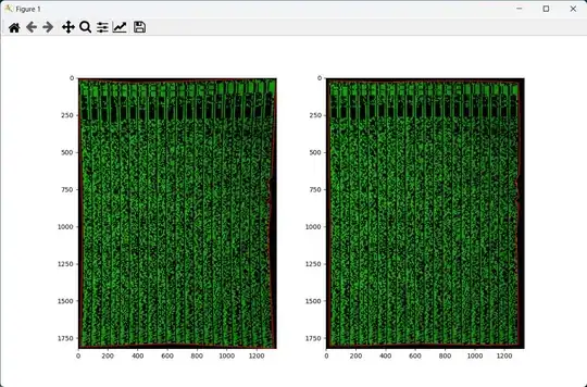
I have the following image which is computer generated

It is fed as an input to an optical experiment results in the following image:

As you can tell the image has a double concave effect due to the lens system being used.

I need to be able to restore the image without distortion and compare it with the original image. I'm new to image processing and I came across two useful python packages:

https://pypi.org/project/defisheye/

The defisheye was quite straight forward for me to use (script below) but i'm not able to achieve the optimal result so far.

from defisheye import Defisheye

dtype = 'linear'
format = 'fullframe'
fov = 11
pfov = 10

img = "input_distorted.jpg"
img_out = "input_distorted_corrected.jpg"

obj = Defisheye(img, dtype=dtype, format=format, fov=fov, pfov=pfov)

# To save image locally 
obj.convert(outfile=img_out)

Seconly from opencv: https://docs.opencv.org/4.x/dc/dbb/tutorial_py_calibration.html The camera calibration tutorial is way out of my knowledge. If someone could assure me if that's the way to go i can start digging in deeper. Really appreciate any suggestions.

Answer 1

If you have access to camera simply calibrate it but if you have no choice, the best way is using a software to do it manually. here I used GIMP to remove the lens effect.

If you have to do it pragmatically you have 2 ways to do it.

First: you can automate GIMP and write a script to do the thing.

Second: find the best coefficients for your camera in OpenCV. here I wrote a script that helps you to find coefficients by test and trial.

import cv2
import numpy as np
import matplotlib.pyplot as plt

src = cv2.imread("camera.jpg")

# convert image to graysclae
src_gray = cv2.cvtColor(src, cv2.COLOR_BGR2GRAY)
height, width = src_gray.shape

# set camera matrix ceofs
focal_lenght_x = 1000
focal_lenght_y = 1000
optical_center_x = 500
optical_center_y = 1000

# set distortion ceofs
k1 = k2 = 0.02
p1 = p2 = 0
k3 = 0

# create camera, distortion and new camera matrix
cameraMatrix = np.array([[focal_lenght_x,0,optical_center_x],[0,focal_lenght_y,optical_center_y], [0,0,1]])
distCoeffs = np.array([[k1, k2, p1, p2, k3]])
newcameramatrix, _ = cv2.getOptimalNewCameraMatrix(
    cameraMatrix, distCoeffs, (width, height), 1, (width, height)
)

# blur image and find contours
src_blur = cv2.blur(src_gray,(13,13))
ret, thresh = cv2.threshold(src_blur, 2, 255, 0)
contours, hierarchy = cv2.findContours(thresh, cv2.RETR_TREE, cv2.CHAIN_APPROX_SIMPLE)

# find the biggest contour by area
c = max(contours, key = cv2.contourArea)
# reduce number of points in contour
epsilon = 0.003*cv2.arcLength(c,True)
approx = cv2.approxPolyDP(c,epsilon,True)
# draw biggest contour
cv2.drawContours(src, [approx], -1, (255,0,0), 3)

# undistor image
undistorted_image = cv2.undistort(
    src, cameraMatrix, distCoeffs, None, newcameramatrix
)

# show original image and undistorted image with contour
fig = plt.figure()
ax1 = fig.add_subplot(1,2,1)
ax1.imshow(src)
ax2 = fig.add_subplot(1,2,2)
ax2.imshow(undistorted_image)
plt.show()

this code draws the biggest contour in the image and shows the image before and after undistortion. you have to find the best values to make the contour look like a rectangle.

You just need to change focal length, optical center, k1, k2, k3, p1 and p2 to reach the best result.

When you find the best values, use them to make your final image.

undistorted_image = cv2.undistort(
    src_gray, cameraMatrix, distCoeffs, None, newcameramatrix
)
src_blur = cv2.blur(undistorted_image,(3,3))
ret, thresh = cv2.threshold(src_blur, 70, 255, 0)
cv2.imwrite("calibrated.png", thresh)

this is the output that I got with the current coefficients.

Answer 2

Idea

Calculate complete lookup tables that model the warp (for cv::remap).

Competing Ideas

I chose a lookup table. Other approaches might estimate lens distortion coefficients, but those would then also need to estimate or assume a fixed pose for the reference pattern.

I looked into fitting a lens distortion model to matched features. It might be doable but (1) calibrateCamera didn't like the single image and kept producing junk (it won't take "guesses" for rvec and tvec) (2) I wasn't inclined to set up the equations for an explicit optimization that would include assumptions about the "3D pose" of the reference pattern, which is how one could form a lens model from this data.

One could set up some gradient descent to optimize lens distortion parameters, given some "experimental setup". I was also not inclined to set that up and come up with good ranges for the delta on each coefficient to use during GD, or to even come up with some kind of learning rate. Getting that to converge seemed more trouble than the optical flow approach below.

Approach

• initialize using homography from feature matching
• refine alignment using optical flow

Results

(1) unwarped, brightness adjusted a little (2) per-pixel difference to reference picture

Details

Feature Extraction, Matching, Homography

The standard example code. SIFT or AKAZE. For Lowe's ratio test, I chose a more severe ratio (0.3) to reduce the number of matches. Might not make any real difference to findHomography.

Oh, also, I took just the green channel of the warped image, and also stretched its values to 0.2 and 0.8 quantile levels.

# H mapping ref to warped image
[[  3.80179   0.02005 -22.76224]
 [ -0.08005   3.88306  13.52028]
 [ -0.00008   0.00003   1.     ]]

You see, in the center it's fairly good already, but only there.

Look-up Tables for cv::remap()

totalmap = np.empty((refheight, refwidth, 2), dtype=np.float32)
totalmap[:,:,1], totalmap[:,:,0] = np.indices((refheight, refwidth))
totalmap = cv.perspectiveTransform(totalmap, H)

I also scaled the reference image up by 3 (nearest neighbor) and wrapped that scaling into the homography matrix. H = H @ inv(np.diag((3.0, 3.0, 1.0))). Helps with looking at things.

Applying current lookup tables:

output = cv.remap(src=imwarped, map1=totalmap, map2=None, interpolation=cv.INTER_CUBIC)

Zero-th iteration (ref, diff, unwarped/output):

Optical Flow

dis = cv.DISOpticalFlow_create(cv.DISOPTICAL_FLOW_PRESET_MEDIUM)

Calculate flow:

flow = dis.calc(I0=imref, I1=output, flow=None)

Note that this is calculated using output, which results from using the current lookup table.

Magnitude of the first iteration of flow:

# applies the increment
totalmap += flow

# keeps the warp reasonably smooth
totalmap = cv.stackBlur(totalmap, (31,31))

first iteration of flow:

second iteration of flow:

Result

Note that the warp map only has reasonably valid values where the images actually have texture. Outside of the pattern, there is no texture, so the values there don't map sensibly.

Ideally, this cross-section would be a straight diagonal, mapping each X value in the reference space to an increasing X value from the warped image. On the borders, it can't determine this, so you get it leveling off. This is in part happening due to the lowpass (stackBlur), but really, there's no support for any sensible values there.

The lowpass also causes some warping inside of textured areas that are near the borders (to untextured area). This effect can be reduced if the last increment (totalmap += flow) isn't lowpassed, or lowpassed less severely than all the previous ones.

Result, Caveats

The result is an xymap suitable for cv::remap(). You can save and load it and apply it to whatever images you like. It'll remove the lens distortion and whatever other spatial effects.

Optical flow can do weird things, just warp the image in ways that aren't well supported by the data. That is one reason why I apply a lowpass, to keep it kinda straight. I also lowpass both images before passing them to optical flow calculation. That helps it not get caught on aliasing effects of the resampling.

Answer 3

I'm going to make the following assumptions:

• You have complete control of the input image
• Displaying an image and capturing its output is relatively fast
• Each "pixel" in the display can only ever be completely on or completely off
• Your goal is to validate that the image displayed matches the data

A solution to this problem that avoids intense computation or lens models could work by calibrating the relationship between each input pixel and the output image separately. A procedure to do this may look like the following:

1. For each pixel generate a calibration image that is completely off except for the pixel being calibrated
2. Capture an image of the output
3. Use that image to determine where the input pixel shows up in the output image This could use several methods:
   • finding the location of the pixel (mean of the locations of the bright pixels in the output image)
   • finding the region in the output image where the input pixel shows up ( a list of all the bright output pixels in each calibration image, or a polygon containing them)
   • storing all the calibration images and decomposing future images in terms of additive combinations of the calibration images