With a logistic regression using glm, the term on the left-hand side of the equation can either be a TRUE / FALSE (or 1 / 0) variable indicating presence / absence, or it can be a two-column matrix indicating the number of positive / negative cases.
From the ?glm documents:
For binomial and quasibinomial families the response can also be specified as a factor (when the first level denotes failure and all others success) or as a two-column matrix with the columns giving the numbers of successes and failures.
If we look at the description of the boot::downs.bc data set, it tells us that the variables are:
age The average age of all mothers in the age category.
m The total number of live births to mothers in the age category.
r The number of cases of Down's syndrome.
So the correct formula would be
mod <- glm(cbind(r, m - r) ~ age, family = binomial, data = boot::downs.bc)
Which results in the following model, showing a highly significant increase in the probability of Down's syndrome as maternal age increases:
summary(mod)
#>
#> Call:
#> glm(formula = cbind(r, m - r) ~ age, family = binomial, data = boot::downs.bc)
#>
#> Deviance Residuals:
#>     Min       1Q   Median       3Q      Max
#> -3.4127  -1.9446   0.5464   2.1361   4.7681
#>
#> Coefficients:
#>               Estimate Std. Error z value Pr(>|z|)
#> (Intercept) -10.563690   0.214485  -49.25   <2e-16 ***
#> age           0.137579   0.006474   21.25   <2e-16 ***
#> ---
#> Signif. codes:  0 '***' 0.001 '**' 0.01 '*' 0.05 '.' 0.1 ' ' 1
#>
#> (Dispersion parameter for binomial family taken to be 1)
#>
#>     Null deviance: 625.21  on 29  degrees of freedom
#> Residual deviance: 184.03  on 28  degrees of freedom
#> AIC: 326.91
#>
#> Number of Fisher Scoring iterations: 5
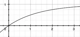
And we can see what this looks like using predict and plot:
plot(predict(mod, newdata = list(age = 16:50), type = 'response'), type = 'l',
     ylab = "Probability of Down's syndrome per live birth",
     xlab = 'Maternal age')
Created on 2023-02-09 with reprex v2.0.2
