How to get connected components label in a binary image?

Question

I've a binary image where removing green dot gets me separate line segments. I've tried using label_components() function from Julia but it labels only verticall joined pixels as one label. I'm using

using Images
img=load("current_img.jpg")
img[findall(img.==RGB(0.0,0.1,0.0))].=0 # this makes green pixels same as background, i.e. black
labels = label_components(img)

I'm expecteing all lines which are disjoint to be given a unique label (as was a funciton in connected component labeling in matlab, but i can't find something similar in julia)

Answer 1

Since you updated the question and added more details to make it clear, I decided to post the answer. Note that this answer utilizes some of the functions that I wrote here; so, if you didn't find documentation for any of the following functions, I refer you to the previous answer. I operated on several examples and brought the results in the continue.
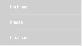
Let's begin with an image similar to the one you brought in the question and perform the entire operation from the scratch. for this, I drew the following:

I want to perform a segmentation process on it and labelize each segment and highlight the segments using the achieved labels.
Let's define the functions:

using Images
using ImageBinarization

function check_adjacent(
  loc::CartesianIndex{2},
  all_locs::Vector{CartesianIndex{2}}
  )

  conditions = [
    loc - CartesianIndex(0,1) ∈ all_locs,
    loc + CartesianIndex(0,1) ∈ all_locs,
    loc - CartesianIndex(1,0) ∈ all_locs,
    loc + CartesianIndex(1,0) ∈ all_locs,
    loc - CartesianIndex(1,1) ∈ all_locs,
    loc + CartesianIndex(1,1) ∈ all_locs,
    loc - CartesianIndex(1,-1) ∈ all_locs,
    loc + CartesianIndex(1,-1) ∈ all_locs
  ]

  return sum(conditions)
end;

function find_the_contour_branches(img::BitMatrix)
  img_matrix = convert(Array{Float64}, img)
  not_black = findall(!=(0.0), img_matrix)
  contours_branches = Vector{CartesianIndex{2}}()
  for nb∈not_black
    t = check_adjacent(nb, not_black)
    (t==1 || t==3) && push!(contours_branches, nb)
  end
  return contours_branches
end;

"""
  HighlightSegments(img::BitMatrix, labels::Matrix{Int64})

Highlight the segments of the image with random colors.

# Arguments
- `img::BitMatrix`: The image to be highlighted.
- `labels::Matrix{Int64}`: The labels of each segment.

# Returns
- `img_matrix::Matrix{RGB}`: A matrix of RGB values.
"""
function HighlightSegments(img::BitMatrix, labels::Matrix{Int64})
  colors = [
    # Create Random Colors for each label
    RGB(rand(), rand(), rand()) for label in 1:maximum(labels)
  ]

  img_matrix = convert(Matrix{RGB}, img)

  for seg∈1:maximum(labels)
    img_matrix[labels .== seg] .= colors[seg]
  end

  return img_matrix
end;

"""
  find_labels(img_path::String)

Assign a label for each segment.

# Arguments
- `img_path::String`: The path of the image.

# Returns
- `thinned::BitMatrix`: BitMatrix of the thinned image.
- `labels::Matrix{Int64}`: A matrix that contains the labels of each segment.
- `highlighted::Matrix{RGB}`: A matrix of RGB values.
"""
function find_labels(img_path::String)
  img::Matrix{RGB} = load(img_path)
  gimg = Gray.(img)
  bin::BitMatrix = binarize(gimg, UnimodalRosin()) .> 0.5
  thinned = thinning(bin)
  contours = find_the_contour_branches(thinned)
  thinned[contours] .= 0
  labels = label_components(thinned, trues(3,3))
  highlighted = HighlightSegments(thinned, labels)

  return thinned, labels, highlighted
end;

The main function in the above is find_labels which returns

1. The thinned matrix.
2. The labels of each segment.
3. The highlighted image (Matrix, actually).

First, I load the image, and binarize the Gray scaled image. Then, I perform the thinning operation on the binarized image. After that, I find the contours and the branches using the find_the_contour_branches function. Then, I turn the color of contours and branches to black in the thinned image; this gives me neat segments. After that, I labelize the segments using the label_components function. Finally, I highlight the segments using the HighlightSegments function for the sake of visualization (this is the bonus :)).
Let's try it on the image I drew above:

result = find_labels("nU3LE.png")

# you can get the labels Matrix using `result[2]`
# and the highlighted image using `result[3]`
# Also, it's possible to save the highlighted image using:
save("nU3LE_highlighted.png", result[3])

The result is as follows:

Also, I performed the same thing on another image:

julia> result = find_labels("circle.png")

julia> result[2]
14×16 Matrix{Int64}:
 0  0  0  0  0  0  0  0  0  0  0  0  0  0  0  0
 0  0  0  0  0  0  0  0  0  0  0  0  0  0  0  0
 0  0  0  0  0  0  0  0  0  4  0  0  0  0  0  0
 0  0  0  0  0  0  0  0  0  4  0  0  0  0  0  0
 0  0  0  0  0  0  0  0  0  4  0  0  0  0  0  0
 0  0  0  0  0  0  0  0  0  4  0  0  0  0  0  0
 0  1  1  0  0  0  3  3  0  0  0  5  5  5  0  0
 0  0  0  0  2  0  0  0  0  0  0  0  0  0  0  0
 0  0  0  0  2  0  0  0  0  0  0  0  0  0  0  0
 0  0  0  0  2  0  0  0  0  0  0  0  0  0  0  0
 0  0  0  0  2  0  0  0  0  0  0  0  0  0  0  0
 0  0  0  0  2  0  0  0  0  0  0  0  0  0  0  0
 0  0  0  0  0  0  0  0  0  0  0  0  0  0  0  0
 0  0  0  0  0  0  0  0  0  0  0  0  0  0  0  0

As you can see, the labels are pretty clear. Now let's see the results of performing the procedure in some examples in one glance:

Original Image	Labeled Image