Logistic function settings in r

Question

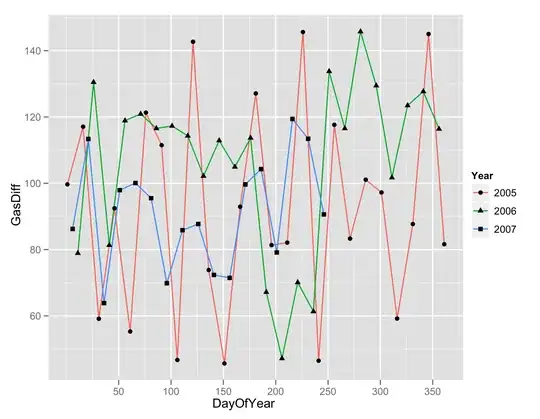
After I made a ggplot of my data

I'd like to adjust each curve with a function. I first adjust with nls function, but for the dark blue one, it doesn't work, and it's obvious when we see the curve shape.
So I want to make a logistic function because of the sigmoid shape, but it doesn't work again. Here is my code, with my starting values:

    start.values <- list(gm=0.6, k=0.8)
    nls4 = nls(growth_rate ~ gm/(1+(exp(-0.8*(quantity-k)))), data = pr28S, start=start.values)

gm is the maximum value of the curve, k is the x value of the sigmoid's midpoint and 0.8 is the logistic growth rate. quantity is my x axis and growth_rate my y axis.

I tried different starting values and change the 0.8 value between 0.5 and 2 but it never work. I have different errors like :

'Error in nls(growth_rate ~ gm/(1 + (exp(-0.8 * (quantity - k)))), data = pr28S, : the step 0.000488281 is lower than'minFactor' of 0.000976562'

or also: 'singular gradient'

How can I adjust my curve pls ?

EDIT : Here is my data for the 28S curve :

structure(list(name = c("J4_S01AC", "J4_S01CC", "J4_S01EC", "J4_S01FC", 
"J4_S03BC", "J4_S03CC", "J4_S03DC", "J4_S03EC", "J4_S03FC", "J4_S06AC", 
"J4_S06DC", "J4_S06EC", "J4_S06FC", "J4_S06KC", "J4_S06MC", "J4_S06NC", 
"J4_S09AC", "J4_S09BC", "J4_S09CC", "J4_S09DC", "J4_S03AM", "J4_S03BM", 
"J4_S03CM", "J4_S15AM", "J4_S15BM", "J4_S15CM", "J4_S15DM", "J4_S01AAC"
), day = c("J4", "J4", "J4", "J4", "J4", "J4", "J4", "J4", "J4", 
"J4", "J4", "J4", "J4", "J4", "J4", "J4", "J4", "J4", "J4", "J4", 
"J4", "J4", "J4", "J4", "J4", "J4", "J4", "J4"), quality = c("S", 
"S", "S", "S", "S", "S", "S", "S", "S", "S", "S", "S", "S", "S", 
"S", "S", "S", "S", "S", "S", "S", "S", "S", "S", "S", "S", "S", 
"S"), quantity = c(0.1, 0.1, 0.1, 0.1, 0.3, 0.3, 0.3, 0.3, 0.3, 
0.6, 0.6, 0.6, 0.6, 0.6, 0.6, 0.6, 0.9, 0.9, 0.9, 0.9, 0.3, 0.3, 
0.3, 1.5, 1.5, 1.5, 1.5, 0.1), qual_quant = c("S01", "S01", "S01", 
"S01", "S03", "S03", "S03", "S03", "S03", "S06", "S06", "S06", 
"S06", "S06", "S06", "S06", "S09", "S09", "S09", "S09", "S03", 
"S03", "S03", "S15", "S15", "S15", "S15", "S01"), temperature = c(28, 
28, 28, 28, 28, 28, 28, 28, 28, 28, 28, 28, 28, 28, 28, 28, 28, 
28, 28, 28, 28, 28, 28, 28, 28, 28, 28, 28), time = c(101, 101, 
101, 101, 101, 101, 101, 101, 101, 101, 101, 101, 101, 101, 101, 
101, 102, 102, 102, 102, 107.5, 107.5, 107.5, 107.5, 107.5, 107.5, 
107.5, 109), size = c(1344.366, 1291.962, 1304.811, 1128.264, 
1286.151, 1358.421, 1396.671, 1353.076, 1505.565, 1297.17, 0, 
1243.029, 1323.85, 1368.364, 1506.396, 0, 1663.735, 1632.28, 
2115.303, 1921.46, 1506.581, 1501.196, 1370.99, 1870.489, 1941.425, 
1942.186, 1827.395, 1336.588), weight = c(11, 16, 10, 10, 12, 
12, 13, 16, 14, 12, 11, 12, 10, 10, 15, 25, 46, 35, 66, 46, 20, 
16, 15, 49, 73, 63, 60, 11), growth_rate = c(0.0378568479840844, 0.126892202895244, 
0.0152090656484838, 0.0152090656484838, 0.0585326533474545, 0.0585326533474545, 
0.0775525505364441, 0.126892202895244, 0.0951622248242906, 0.0585326533474545, 
0.0378568479840844, 0.0585326533474545, 0.0152090656484838, 0.0152090656484838, 
0.111556439370444, 0.232939774941222, 0.374129156018743, 0.309825356331568, 
0.459072793066665, 0.374129156018743, 0.169037347727828, 0.119219651092275, 
0.104811166292231, 0.369092608582107, 0.458090402952369, 0.425199566970549, 
0.414306966296783, 0.0350783637283718), color = c("28S", "28S", 
"28S", "28S", "28S", "28S", "28S", "28S", "28S", "28S", "28S", 
"28S", "28S", "28S", "28S", "28S", "28S", "28S", "28S", "28S", 
"28S", "28S", "28S", "28S", "28S", "28S", "28S", "28S")), row.names = c(NA, 
-28L), class = c("tbl_df", "tbl", "data.frame"))

I just edited my post ! – Nathan FRIZOT Jul 16 '22 at 07:39 — Nathan FRIZOT, Jul 16 '22 at 07:39

Dave2e · Answer 1 · 2022-07-16T14:34:14.000

The problem you were facing was your model was not sufficiently accurate enough to describe the data. nls was was reducing the step size faster then there was improvement in the optimization function thus generating the error. The error tolerance for the fit was too large.
I suggest adding the "trace =TRUE" option to the function is see the intermediate values and whether the fitting is matching expectations.

If you define an additional model parameter to replace the -.8 multiplication factor then you obtain a much better model.

#need additiona parameters in the model
start.values <- list(gm=0.43, k=0.73, i=8.6)
#set trace=true to see the intermediate values
#only way to understand if nls is approaching the correct values
nls4 = nls(growth_rate ~ gm/(1+(exp(-i*(quantity-k)))), data = df, start=start.values, trace =TRUE)  

plot(x=df$quantity, y=df$growth_rate)

#define function for plotting
# this is needed over predict to try out intermediate values 
#predict does not work when nls does not produce a final answer
fn<- function(x) {
   gm <-coefficients(nls4)[1]  #.43
   k <- coefficients(nls4)[2]  #.73  
   i<- coefficients(nls4)[3]   #8.67
   
   gm/(1+(exp(-i*(x-k))))
}

x<-seq(0.1, 1.5, 0.1)
plot(x=df$quantity, y=df$growth_rate)
lines(x, fn(x), col="blue")

Logistic function settings in r

1 Answers1