How to inter cumulative sums between two dates and period for individual days?

Question

I would like to extrapolate the sums between two days into daily values. The counts represent the cumulative sums collected up to certain day: Let's say, at day X there is XX apples fallen on the ground. How many apples fell on the ground daily and per different trees? The average apples a day to certain date (DOY) should equal the number of trees in DOY divided by number of previous days without any record (NA).

In R, I think I need to first recreate the full date range I wish to recalculate the daily values into (2:20). Then merge it with original data. But how to do the interpolate between the dates? The beginning would be then 0 count at DOY 2 (beggining of time series) interpolated until the counts on the first recorded DOY. The fnal values can be only NA, as I do not have any data there (and I can't assume there will be increasing apples of falling apples at the end of season, rather there will be less of them). Scale 2:20 is only used here to understand the process. My original data extends to DOY 270.

Here is my dummy example:

dd <- data.frame(cumsum = c(4, 12, 14.5,
                           8, 15, 20,
                           10, 20, 40),
                 doy = c(4, 10, 15, # DOY = day of the year
                         5, 11, 14,
                         5, 10, 15),
                 gp = rep(c('a', 'b', 'd'), each = 3)) # group

doy_df = data.frame(doy = rep(c(2:20), 3),
                    gp = rep(c('a', 'b', 'd'), each = 19))

# complete the df by wished doy
dd %>% 
  right_join(doy_df) %>% 
  arrange(gp, doy)

How to get the daily value, while accunting for different groups? Here is an example in python, but how to make it in R?

Desired outcome:

  doy_val doy gp
1      2      2  a
2      4      3  a
3      6      4  a    # counted doy
4      7      5  a
5      8      6  a
6      9      7  a
7      10     8  a
8      11     9  a
9      12    10  a  # counted doy
10     12.5  11  a
11     13    12  a
12     13.5  13  a
13     14    14  a
14     14.5  15  a  # counted doy
15     NA    16  a
16     NA    17  a
17     NA    18  a
....

Answer 1

We can interpolate fairly easy using splines. To extrapolate we could use a polynomial model. Let's give the data a flag first to keep control of the results.

dd$flag <- 0

Interpolation

To use the individual doy (what actually is it? was day meant?) ranges, we create a data.frame of the respective sequences using do.call (we also could do seq.int(min(x$doy), max(x$doy))) and merge it to the original data. Next we perform a spline interpolation and replace just the NAs.

res1 <- by(dd, dd$gp, \(x) {
  a <- cbind(merge(x[-3], data.frame(doy=do.call(seq.int, as.list(range(x$doy)))), all=TRUE), gp=el(x$gp))
  na <- is.na(a$cumsum)
  int <- with(a, spline(doy, cumsum, n=nrow(a)))$y
  transform(a, cumsum=replace(cumsum, na, int[na]), flag=replace(flag, is.na(flag), 1))
}) |> do.call(what=rbind)
res1
#      doy    cumsum gp
# a.1    4  4.000000  a
# a.2    5  5.333333  a
# a.3    6  6.666667  a
# a.4    7  8.000000  a
# a.5    8  9.333333  a
# a.6    9 10.666667  a
# a.7   10 12.000000  a
# a.8   11 12.500000  a
# a.9   12 13.000000  a
# a.10  13 13.500000  a
# a.11  14 14.000000  a
# a.12  15 14.500000  a
# b.1    5  8.000000  b
# b.2    6  9.166667  b
# b.3    7 10.333333  b
# b.4    8 11.500000  b
# b.5    9 12.666667  b
# b.6   10 13.833333  b
# b.7   11 15.000000  b
# b.8   12 16.666667  b
# b.9   13 18.333333  b
# b.10  14 20.000000  b
# d.1    5 10.000000  d
# d.2    6 12.000000  d
# d.3    7 14.000000  d
# d.4    8 16.000000  d
# d.5    9 18.000000  d
# d.6   10 20.000000  d
# d.7   11 24.000000  d
# d.8   12 28.000000  d
# d.9   13 32.000000  d
# d.10  14 36.000000  d
# d.11  15 40.000000  d

Looks like this:

plot(cumsum ~ doy, res1, type='n')
by(res1, res1$gp, \(x) with(x, points(doy, cumsum, type='b', pch=20, col=flag + 1)))

See this answer for linear interpolation using approx.

Alternatively, if you need the doy at all equal periods, e.g. 2:20, we first follow the same approach, because spline would omit the NAs. At the end we merge the result to an extra data.frame containing the complete period.

res1a <- by(dd, dd$gp, \(x) {
  a <- cbind(merge(x[-3], data.frame(doy=do.call(seq.int, as.list(range(x$doy)))), all=TRUE), gp=el(x$gp))
  na <- is.na(a$cumsum)
  int <- with(a, spline(doy, cumsum, n=nrow(a)))$y
  df <- transform(a, cumsum=replace(cumsum, na, int[na]), flag=replace(flag, is.na(flag), 1))
  merge(df, data.frame(doy=2:20, gp=el(a$gp)), all=TRUE) |> {\(.) .[order(.$doy), ]}()
}) |> do.call(what=rbind)
res1a

head(res1a)
#     doy gp   cumsum flag
# a.1   2  a       NA   NA
# a.2   3  a       NA   NA
# a.3   4  a 4.000000    0
# a.4   5  a 5.712121    1
# a.5   6  a 7.272727    1
# a.6   7  a 8.681818    1

Extrapolation

Similarly we do to to extrapolate, but use a polynomial lm with say degree=2 (but is rather too few, but more won't work with the few available values in this example) and use the predictions,

res2 <- by(dd, dd$gp, \(x) {
  a <- cbind(merge(x[-3], data.frame(doy=2:20), all=TRUE), gp=el(x$gp))
  na <- is.na(a$cumsum)
  int <- predict(lm(cumsum ~ poly(doy, degree=2), x), newdata=a)
  int[int < 0] <- 0  ## to prevent negative values
  transform(a, cumsum=replace(cumsum, na, int[na]), flag=replace(flag, is.na(flag), 1))
}) |> do.call(what=rbind)
res2
#      doy    cumsum flag gp
# a.1    4  4.000000    0  a
# a.2    5  5.333333    1  a
# a.3    6  6.666667    1  a
# a.4    7  8.000000    1  a
# a.5    8  9.333333    1  a
# a.6    9 10.666667    1  a
# a.7   10 12.000000    0  a
# a.8   11 12.500000    1  a
# a.9   12 13.000000    1  a
# a.10  13 13.500000    1  a
# a.11  14 14.000000    1  a
# a.12  15 14.500000    0  a
# b.1    5  8.000000    0  b
# b.2    6  9.166667    1  b
# b.3    7 10.333333    1  b
# b.4    8 11.500000    1  b
# b.5    9 12.666667    1  b
# b.6   10 13.833333    1  b
# b.7   11 15.000000    0  b
# b.8   12 16.666667    1  b
# b.9   13 18.333333    1  b
# b.10  14 20.000000    0  b
# d.1    5 10.000000    0  d
# d.2    6 12.000000    1  d
# d.3    7 14.000000    1  d
# d.4    8 16.000000    1  d
# d.5    9 18.000000    1  d
# d.6   10 20.000000    0  d
# d.7   11 24.000000    1  d
# d.8   12 28.000000    1  d
# d.9   13 32.000000    1  d
# d.10  14 36.000000    1  d
# d.11  15 40.000000    0  d

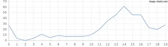
which looks like this:

plot(cumsum ~ doy, res2, type='n')
by(res2, res2$gp, \(x) with(x, points(doy, cumsum, type='b', pch=20, col=flag + 1)))

Note, that inter/extrapolation may be problematic with few data points as in your example, but you might have more in your original data. Also for the extrapolation, you may want to check if there are significant higher polynomials in the groups, to better prevent increasing predictions to the left (see plot). Alternatively we could use non-parametric approaches such as loess.

---

Data

dd <- structure(list(cumsum = c(4, 12, 14.5, 8, 15, 20, 10, 20, 40), 
    doy = c(4, 10, 15, 5, 11, 14, 5, 10, 15), gp = c("a", "a", 
    "a", "b", "b", "b", "d", "d", "d"), flag = c(0, 0, 0, 0, 
    0, 0, 0, 0, 0)), row.names = c(NA, -9L), class = "data.frame")