Option 1 (HSV color space):
If you want to continue using HSV color space robustly, you must check out this post. There you can control the variations across the three channels using trackbars.
Option 2 (LAB color space):
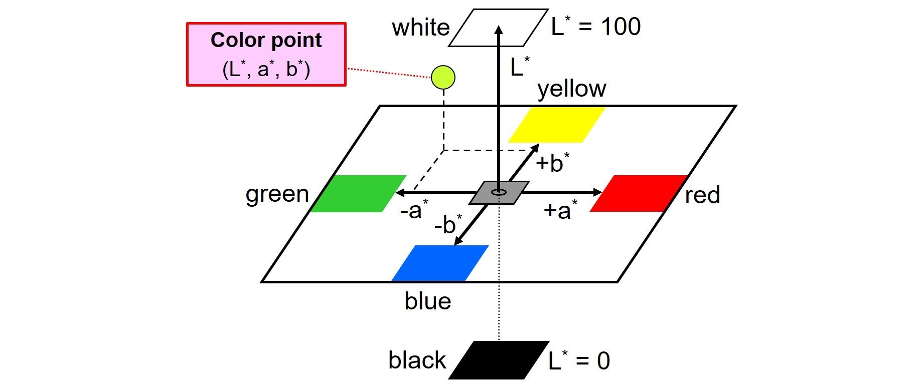
Here I will be using the LAB color space where dominant colors can be segmented pretty easily. LAB space stores image across three channels (1 brightness channel) and (2 color channels):
- L-channel: amount of lightness in the image
- A-channel: amount of red/green in the image
- B-channel: amount of blue/yellow in the image
Since orange is a close neighbor of color red, using the A-channel can help segment it.
Code:
img = cv2.imread('image_path')

# Convert to LAB color space
lab = cv2.cvtColor(img, cv2.COLOR_BGR2LAB)
cv2.imshow('A-channel', lab[:,:,1])

The above image is the A-channel, where the object of interest is pretty visible.
# Apply threshold
th = cv2.threshold(lab[:,:,1],150,255,cv2.THRESH_BINARY)[1]
Why does this work?
Looking at the LAB color plot, the red color is on one end of A-axis (a+) while green color is on the opposite end of the same axis (a-). This means, higher values in this channel represents colors close to red, while the lower values values represents colors close to green.
The same can be done along the b-channel while trying to segment yellow/blue color in the image.
Post-processing:
From here onwards for every frame:
- Identify the largest contour in the binary threshold image
th.
- Mask it over the frame using
cv2.bitwise_and()
Note: this LAB color space can help segment dominant colors easily. You need to test them before using it for other colors.


