We use Excel from Office 365 with a SQL Server 2019 Tabular model
I have a "strange" behaviour of Excel Pivot regarding the level at which calculations are requested from DAX.
We have a measure that behaves differently depending on the granularity level you query it at.
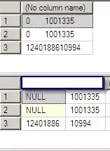
In the example above, the measure is queried at "BRAND_NAME" level with some filters.
The sum of the Brand numbers does not equal the total, which is "fine" as it is a known side effect of that measure in this particular query.
Now, if we add a layer underneath, then the Excel Pivot shows a behaviour that is a problem for us
I'll do my best but it is not easy to explain...
What the Excel pivot is showing us is
- the TOTAL_SALES_UNIT for the Item SAMSUNG "SP 54J8 HFR" (evaluated at ITEM Level)
- the TOTAL_SALES_UNIT for the Item SAMSUNG "TRADE MODEL" (evaluated at ITEM Level)
- the TOTAL_SALES_UNIT for the Brand "OTHERS" (evaluated at BRAND Level, probably because there is no record underneath the "OTHERS" Brand...)
Our measure TOTAL_SALES_UNIT is complicated and coded in such a way that it would return 0 if evaluated at ITEM level under the OTHERS brand...
BUT there is no ITEM under the OTHERS Brand and it looks like Excel Pivot somehow decides to evaluate our measure at the Brand level instead of the Item level...
Running a similar request under SSMS returns the result we were expecting
Question: Is there a way in Excel that we could control this pivot table behaviour?


