1

How does one plot the solutions to a set of equations in Mathematica? Even if there are only two variables, these equations are sufficiently complicated that they cannot be rearranged so that one of the variables can be set equal to a function of the other (and thus be of the correct form for Plot).

The specific example I am interested in is the following:

  • Fix a b in (0,1).
  • Let g >= 1 and d >= 1 vary.
  • Then there is a unique x (which happens to be in (0,1]) such that x = [(b x + 1) / (x + g)]^d (proof omitted).
  • I want a plot of pairs (d, g) that (1 - b g) x d / [(b x + 1) (x + g)] = 1.
Tyson Williams
  • 1,630
  • 15
  • 35
  • 1
    Can you give a simplified example of your equations? How many variables and how many equations are there? – Simon Jul 27 '11 at 00:41
  • Each eqn is a function of two variables, right? You could Plot3D[] that function. You can also Plot3D several eqns in the same plot, though depending on what the equations are like it may or may not be readable/useful – Daniel Chisholm Jul 27 '11 at 01:32
  • @Simon provided specific example. – Tyson Williams Aug 01 '11 at 19:26
  • @Daniel Chisholm One can solve a variable and reduce the problem to two variables. However, this is not a 3D problem. Either a 2D point satisfies the equation or it does not, hence the "third dimension" is only a binary on/off. – Tyson Williams Aug 01 '11 at 19:26
  • @Tyson If you have `lefthandside(x,y) = righthandside(x,y)` then you're interested in the 3D graph of `Z = lefthandside(x,y)-righthandside(x,y)`, which is definitely not just 0 or 1. You're interested in the slice of the graph where Z=0 though. I'm sure you can take it from here; I haven't used mathematica in a long time – Rag Aug 01 '11 at 21:00
  • @Brian Gordon Of course one reason about a lower dimension in terms of a higher one, but without some justification, this is pedantic. Generalization for the sake of generalization should be avoided. – Tyson Williams Aug 03 '11 at 16:34

2 Answers2

3

You want to use ContourPlot.

http://reference.wolfram.com/mathematica/ref/ContourPlot.html

You can also use ImplicitPlot, but it's deprecated:

http://reference.wolfram.com/legacy/v5_2/Add-onsLinks/StandardPackages/Graphics/ImplicitPlot.html

Rag
  • 6,405
  • 2
  • 31
  • 38
  • Please correct me if I am wrong, but it appears that both functions only work with a single equation. – Tyson Williams Jul 27 '11 at 00:26
  • @Tyson take a look at the third command in the yellow box at the top of ContourPlot – Rag Jul 27 '11 at 12:14
  • Yes, but under "More Information," it says "ContourPlot superimposes the contour lines associated with all of the equalities" about the third command, which means that the countour contains a point if it is a solution to ANY of the equations instead of what I am looking for, which is the set of points that are solutions to ALL equations. – Tyson Williams Aug 01 '11 at 19:11
2

I imagine you're looking for some elegant method, but for now here's how to brute-force it:

Clear[findx];findx[d_,g_,b_]:=x/.First@FindRoot[x\[Equal]((b x+1)/(x+g))^d,{x,0,1},PrecisionGoal\[Rule]3]
ClearAll[plotQ];
plotQ[d_,g_,b_,eps_]:=Module[
    {x=findx[d,g,b]},
    Abs[(1-b g) x d/((b x+1) (x+g))-1.]<eps]

tbl=Table[{d,g,plotQ[d,g,.1,.001]},{d,4,20,.05},{g,1,1.12,.001}];

(this should take of the order of 10s). Then draw the points as follows:

Reap[
    Scan[
        If[#[[3]] == True,
            Sow@Point[{#[[1]], #[[2]]}]] &,
            Flatten[tbl, 1]]] // Last // Last // 
 Graphics[#, PlotRange -> {{1, 20}, {1, 1.1}}, Axes -> True,
    AspectRatio -> 1, AxesLabel -> {"d", "g"}] &

enter image description here

Painfully ugly way to go about it, but there it is.

Note that I just quickly wrote this up so I make no guarantees it's correct!

EDIT: Here is how to do it with only providing b and a stepsize for d:

Clear[findx]; 
findx[d_, g_, b_] := 
 x /. First@
   FindRoot[x \[Equal] ((b x + 1)/(x + g))^d, {x, 0, 1}, 
    PrecisionGoal \[Rule] 3]
ClearAll[plotQ];
plotQ[d_, g_, b_, eps_] := 
 Module[{x = findx[d, g, b]}, 
  Abs[(1 - b g) x d/((b x + 1) (x + g)) - 1.] < eps]

tbl = Table[{d, g, plotQ[d, g, .1, .001]}, {d, 4, 20, .05}, {g, 1, 
    1.12, .001}];

ClearAll[tmpfn];
tmpfn[d_?NumericQ, g_?NumericQ, b_?NumericQ] := 
 With[{x = findx[d, g, b]},
    (1 - b g) x d/((b x + 1) (x + g)) - 1.
  ]

then

stepsize=.1

(tbl3=Table[
    {d,g/.FindRoot[tmpfn[d,g,.1]\[Equal]0.,
        {g,1,2.},PrecisionGoal\[Rule]2]},
    {d,1.1,20.,stepsize}]);//Quiet//Timing

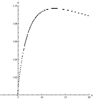
ListPlot[tbl3,AxesLabel\[Rule]{"d","g"}]

giving

enter image description here

acl
  • 6,490
  • 1
  • 27
  • 33
  • Don't worry, I am not trying to win a beauty contest here. Also, this is the type of curve that I expect. However, I can't tell what value of *b* you selected for this plot. Do you perhaps plot all the *(d, g, b)* triples but throw away the *b* coordinate? – Tyson Williams Aug 02 '11 at 12:45
  • @Tyson `b` is the third argument of `plotQ`; if you look at what `tbl` is set to, `b=.1`. By the way, the way I wrote this is fairly hard to understand (it's a quick and dirty implementation that I wrote up without thinking much). If you do not understand something go ahead and ask (I really should have cleaned it up but did not have much time). – acl Aug 02 '11 at 12:54
  • Ok, what about this improvement? You say that this is just brute force. It seems like you just look over all pairs *(d, g)* (for a fixed *b*) within a 2D lattice and plot the "True" points. As the plot suggests, I expect the "True" points to be form a function in *d*. Can you improve it so that only the range and step size for *d* need to be given? – Tyson Williams Aug 02 '11 at 13:19
  • @Tyson Yes you understood correctly: I simply calculate which points on a lattice are `True`, then plot them. – acl Aug 02 '11 at 13:27
  • @Tyson see edit. Have you actually trying simplifying this analytically? – acl Aug 02 '11 at 13:59
  • Not analytically, only symbolically. – Tyson Williams Aug 02 '11 at 14:20
  • @acl let us [continue this discussion in chat](http://chat.stackoverflow.com/rooms/2066/discussion-between-tyson-williams-and-acl) – Tyson Williams Aug 02 '11 at 14:42
  • @Tyson I did; in any case I found a stupid mistake (I left in an `Abs`; I removed it and now it works OK for all your values) – acl Aug 02 '11 at 15:01
  • I think the second parameter of FindRoot should be {x, 0.5, 0, 1} (where 0.5 can be any value between 0 and 1) in order to find a root for x between 0 and 1. – Tyson Williams Aug 04 '11 at 22:27
  • @Tyson yes that restricts the range. I was simply giving initial conditions and trying to avoid using derivatives (assuming it would be faster, although in the end I did not check) – acl Aug 04 '11 at 22:47
  • The problem is that I need an x in [0,1]. This seems to happen when plotting g vs d, but my friend wanted to see g / x vs d and I think x's outside of [0,1] were being returned. – Tyson Williams Aug 05 '11 at 02:23
  • @Tyson does using `FindRoot` like you said, eg, `FindRoot[Cos[x], {x, 0.5, 0, 1}]`, not always return x in `[0,1]`? – acl Aug 05 '11 at 09:11
  • That is what the documentation says, so it probably does. In our graphs, since we are dividing by x, which is very small, so slight differences in the returned value cause very big differences. This specific problem is probably no longer of great concern because the g vs d graphs indicate that our approach to solve the problem won't work. Thanks again for all the help. – Tyson Williams Aug 09 '11 at 23:10