3

I am working on finding the frequencies from a given dataset and I am struggling to understand how np.fft.fft() works. I thought I had a working script but ran into a weird issue that I cannot understand.

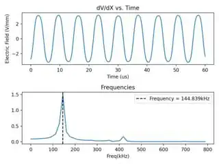
I have a dataset that is roughly sinusoidal and I wanted to understand what frequencies the signal is composed of. Once I took the FFT, I got this plot:

Time plot

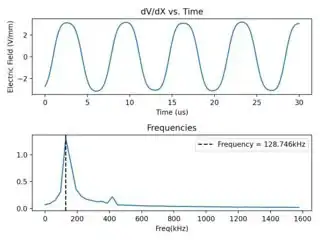
However, when I take the same dataset, slice it in half, and plot the same thing, I get this:

FFT plot

I do not understand why the frequency drops from 144kHz to 128kHz which technically should be the same dataset but with a smaller length.

I can confirm a few things:

  1. Step size between data points 0.001
  2. I have tried interpolation with little luck.
  3. If I slice the second half of the dataset I get a different frequency as well.
  4. If my dataset is indeed composed of both 128 and 144kHz, then why doesn't the 128 peak show up in the first plot?

What is even more confusing is that I am running a script with pure sine waves without issues:

T = 0.001
fs = 1 / T
def find_nearest_ind(data, value):
    return (np.abs(data - value)).argmin()
x = np.arange(0, 30, T)
ff = 0.2
y = np.sin(2 * ff * np.pi * x)
x = x[:len(x) // 2]
y = y[:len(y) // 2]

n = len(y) # length of the signal
k = np.arange(n)
T = n / fs
frq = k / T * 1e6 / 1000 # two sides frequency range
frq = frq[:len(frq) // 2] # one side frequency range

Y = np.fft.fft(y) / n # dft and normalization
Y = Y[:n // 2]

frq = frq[:50]
Y = Y[:50]

fig, (ax1, ax2) = plt.subplots(2)
ax1.plot(x, y)
ax1.set_xlabel("Time (us)")
ax1.set_ylabel("Electric Field (V / mm)")
peak_ind = find_nearest_ind(abs(Y), np.max(abs(Y)))
ax2.plot(frq, abs(Y))
ax2.axvline(frq[peak_ind], color = 'black', linestyle = '--', label = F"Frequency = {round(frq[peak_ind], 3)}kHz")
plt.legend()
plt.xlabel('Freq(kHz)')
ax1.title.set_text('dV/dX vs. Time')
ax2.title.set_text('Frequencies')
fig.tight_layout()
plt.show()
Mad Physicist
  • 107,652
  • 25
  • 181
  • 264
pmoh
  • 81
  • 8
  • The maximum frequency should be the same in all cases: if you sample at 1kHz, your Nyquist is at 500Hz, no matter how many samples you have. So start by looking there – Mad Physicist Dec 17 '20 at 06:55
  • Frequency axis: `np.linspace(0, 1, N) / T ` – Mad Physicist Dec 17 '20 at 06:58
  • 1
    `find_nearest_ind(abs(Y), np.max(abs(Y)))` is just `np.abs(Y).argmax()`. You don't need the function at all. – Mad Physicist Dec 17 '20 at 07:17
  • Your period is 6-7microseconds in the plots. So clearly the frequency should be between 140 and 160 kHz – Mad Physicist Dec 17 '20 at 07:20
  • The frequency is in the correct range but I am just curious about the shift depending on the size of the dataset. I am clearly doing something wrong. I tried using ```np.linspace(0,1,N)/T``` but I am getting similar issues – pmoh Dec 17 '20 at 07:25
  • Just to be clear, removing the lines `x = x[:len(x)//2]; y = y[:len(y)//2]` triggers the shift? – Mad Physicist Dec 17 '20 at 07:44
  • I think I got it. Has to do with sampling resolution – Mad Physicist Dec 17 '20 at 07:45
  • Can you tell me what `frq[peak_ind-1:peak_ind+2]` gives in both cases? – Mad Physicist Dec 17 '20 at 07:46
  • I'll get to a desktop in about 6hrs. Until then it's mobile only. This is a curious problem. – Mad Physicist Dec 17 '20 at 07:49
  • i can try and update my question with the actual dataset and that might help. But to answer your question, for half the dataset i get [ 96.5623793 128.74983906 160.93729883] and for the complete dataset i get [128.74776703 144.84123791 160.93470879] all in kHz – pmoh Dec 17 '20 at 08:06
  • No need. What you have here provides a perfect MCVE. Take a look at your frequency bins. In both cases, the maximum occurs at the bin closest to the true frequency. The shift occurs because your resolution dropped by a factor of 2 and fs is not a multiple of ff. – Mad Physicist Dec 17 '20 at 16:40
  • Please reinstate the original example. *Never* load a dataset that you don't provide in a code example. It makes the whole thing completely useless. Your original formulation was perfect because you had an MCVE for us to discuss. – Mad Physicist Dec 17 '20 at 16:45
  • I have added back my original example at the end. What you are saying makes sense to me. However, shouldn't that problem go away when I interpolate the smaller dataset to make sure that the step size is 0.001? – pmoh Dec 17 '20 at 18:03
  • The point is that the sine wave frequency of ff can not be represented as an exact multiple of 1kHz. The interpolation does basically nothing. You need to fit a parabola to the peak and find the maximum of that. I'll post an answer in a bit. – Mad Physicist Dec 17 '20 at 18:11
  • 1
    For the purposes of this question, remove the part with the real dataset. Your question should always focus on a single self-contained MCVE, never your real code. – Mad Physicist Dec 17 '20 at 18:29
  • Also, I hope you mean `np.abs` where you say `abs` – Mad Physicist Dec 17 '20 at 18:30
  • I see. Also, yes i do mean np.abs(). Also thank you for your help. – pmoh Dec 17 '20 at 18:44
  • No problem. hopefully my answer is clear enough and you agree with me about what is going on. – Mad Physicist Dec 17 '20 at 20:37

1 Answers1

2

Here is a breakdown of your code, with some suggestions for improvement, and extra explanations. Working through it carefully will show you what is going on. The results you are getting are completely expected. I will propose a common solution at the end.

First set up your units correctly. I assume that you are dealing with seconds, not microseconds. You can adjust later as long as you stay consistent.

Establish the period and frequency of the sampling. This means that the Nyquist frequency for the FFT will be 500Hz:

T = 0.001      # 1ms sampling period
fs = 1 / T     # 1kHz sampling frequency

Make a time domain of 30e3 points. The half domain will contain 15000 points. That implies a frequency resolution of 500Hz / 15k = 0.03333Hz.

x = np.arange(0, 30, T)   # time domain
n = x.size                # number of points: 30000

Before doing anything else, we can define our time domain right here. I prefer a more intuitive approach than what you are using. That way you don't have to redefine T or introduce the auxiliary variable k. But as long as the results are the same, it does not really matter:

F = np.linspace(0, 1 - 1/n, n) / T    # Notice F[1] = 0.03333, as predicted

Now define the signal. You picked ff = 0.2. Notice that 0.2Hz. 0.2 / 0.03333 = 6, so you would expect to see your peak in exactly bin index 6 (F[6] == 0.2). To better illustrate what is going on, let's take ff = 0.22. This will bleed the spectrum into neighboring bins.

ff = 0.22
y = np.sin(2 * np.pi * ff * x)

Now take the FFT:

Y = np.fft.fft(y) / n
maxbin = np.abs(Y).argmax()  # 7
maxF = F[maxbin]             # 0.23333333: This is the nearest bin

Since your frequency bins are 0.03Hz wide, the best resolution you can expect 0.015Hz. For your real data, which has much lower resolution, the error is much larger.

Now let's take a look at what happens when you halve the data size. Among other things, the frequency resolution becomes smaller. Now you have a maximum frequency of 500Hz spread over 7.5k samples, not 15k: the resolution drops to 0.066666Hz per bin:

n2 = n // 2                               # 15000
F2 = np.linspace(0, 1 - 1 / n2, n2) / T   # F[1] = 0.06666
Y2 = np.fft.fft(y[:n2]) / n2

Take a look what happens to the frequency estimate:

maxbin2 = np.abs(Y2).argmax()  # 3
maxF2 = F2[maxbin2]            # 0.2: This is the nearest bin

Hopefully, you can see how this applies to your original data. In the full FFT, you have a resolution of ~16.1 per bin with the full data, and ~32.2kHz with the half data. So your original result is within ~±8kHz of the right peak, while the second one is within ~±16kHz. The true frequency is therefore between 136kHz and 144kHz. Another way to look at it is to compare the bins that you showed me:

full: 128.7 144.8 160.9 half: 96.6 128.7 160.9

When you take out exactly half of the data, you drop every other frequency bin. If your peak was originally closest to 144.8kHz, and you drop that bin, it will end up in either 128.7 or 160.9.

Note: Based on the bin numbers you show, I suspect that your computation of frq is a little off. Notice the 1 - 1/n in my linspace expression. You need that to get the right frequency axis: the last bin is (1 - 1/n) / T, not 1 / T, no matter how you compute it.

So how to get around this problem? The simplest solution is to do a parabolic fit on the three points around your peak. That is usually a sufficiently good estimator of the true frequency in the data when you are looking for essentially perfect sinusoids.

def peakF(F, Y):
    index = np.abs(Y).argmax()
    # Compute offset on normalized domain [-1, 0, 1], not F[index-1:index+2]
    y = np.abs(Y[index - 1:index + 2])
    # This is the offset from zero, which is the scaled offset from F[index]
    vertex = (y[0] - y[2]) / (0.5 * (y[0] + y[2]) - y[1])
    # F[1] is the bin resolution
    return F[index] + vertex * F[1]

In case you are wondering how I got the formula for the parabola: I solved the system with x = [-1, 0, 1] and y = Y[index - 1:index + 2]. The matrix equation is

[(-1)^2 -1  1]   [a]   Y[index - 1]
[   0^2  0  1] @ [b] = Y[index]
[   1^2  1  1]   [c]   Y[index + 1]

Computing the offset using a normalized domain and scaling afterwards is almost always more numerically stable than using whatever huge numbers you have in F[index - 1:index + 2].

You can plug the results in the example into this function to see if it works:

>>> peakF(F, Y)
0.2261613409657391
>>> peakF(F2, Y2)
0.20401580936430794

As you can see, the parabolic fit gives an improvement, however slight. There is no replacement for just increasing frequency resolution through more samples though!
Mad Physicist
  • 107,652
  • 25
  • 181
  • 264
  • This really clarifies a lot of my questions. Thank you for such a detailed response (especially with the explanation of how the frequency bins change)! – pmoh Dec 17 '20 at 23:21
  • @Parashar. I like the Einstein theory of explaining: if you can't explain it to someone else, you don't know it yourself. I'm glad you were able to understand my explanation. I hope it helps you think about FFTs more intuitively. – Mad Physicist Dec 17 '20 at 23:36
  • So I tried both: 1. fitting a parabola to get the true frequency. 2. running my simulation with a finer step size of 1e-5. The parabola gets me closer but not close enough to the true frequency. The finer step size of 1e-5 creates the same issue as before but now the shift is smaller. Also the simulation takes an unreasonable amount of time so its not my first choice. Do you know of any other methods of solving this issue? I can just interpolate the initial dataset to get really a really small T but i am not sure how to pick a value that'll work. – pmoh Dec 18 '20 at 07:36
  • @Parashar. Your best bet is to get `ff` as a multiple of `fs` – Mad Physicist Dec 18 '20 at 11:45