How to plot a Python 3-dimensional level set?

Question

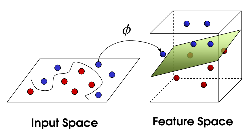
I have some trouble plotting the image which is in my head. I want to visualize the Kernel-trick with Support Vector Machines. So I made some two-dimensional data consisting of two circles (an inner and an outer circle) which should be separated by a hyperplane. Obviously this isn't possible in two dimensions - so I transformed them into 3D. Let n be the number of samples. Now I have an (n,3)-array (3 columns, n rows) X of data points and an (n,1)-array y with labels. Using sklearn I get the linear classifier via

clf = svm.SVC(kernel='linear', C=1000)
clf.fit(X, y)

I already plot the data points as scatter plot via

plt.scatter(X[:, 0], X[:, 1], c=y, s=30, cmap=plt.cm.Paired)

Now I want to plot the separating hyperplane as surface plot. My problem here is the missing explicit representation of the hyperplane because the decision function only yields an implicit hyperplane via decision_function = 0. Therefore I need to plot the level set (of level 0) of an 4-dimensional object.

Since I'm not a python expert I would appreciate if somebody could help me out! And I know that this isn't really the "style" of using a SVM but I need this image as an illustration for my thesis.

Edit: my current "code"

import numpy as np
import matplotlib.pyplot as plt
from sklearn import svm
from sklearn.datasets import make_blobs, make_circles

from tikzplotlib import save as tikz_save

plt.close('all')

# we create 50 separable points
#X, y = make_blobs(n_samples=40, centers=2, random_state=6)
X,  y  = make_circles(n_samples=50, factor=0.5, random_state=4, noise=.05)
X2, y2 = make_circles(n_samples=50, factor=0.2, random_state=5, noise=.08)

X = np.append(X,X2, axis=0)
y = np.append(y,y2, axis=0)

# shifte X to [0,2]x[0,2]
X = np.array([[item[0] + 1, item[1] + 1] for item in X])
X[X<0] = 0.01

clf = svm.SVC(kernel='rbf', C=1000)
clf.fit(X, y)

plt.scatter(X[:, 0], X[:, 1], c=y, s=30, cmap=plt.cm.Paired)


# plot the decision function
ax = plt.gca()
xlim = ax.get_xlim()
ylim = ax.get_ylim()

# create grid to evaluate model
xx = np.linspace(xlim[0], xlim[1], 30)
yy = np.linspace(ylim[0], ylim[1], 30)
YY, XX = np.meshgrid(yy, xx)
xy = np.vstack([XX.ravel(), YY.ravel()]).T
Z = clf.decision_function(xy).reshape(XX.shape)

# plot decision boundary and margins
ax.contour(XX, YY, Z, colors='k', levels=[-1, 0, 1], alpha=0.5, linestyles=['--','-','--'])
# plot support vectors
ax.scatter(clf.support_vectors_[:, 0], clf.support_vectors_[:, 1], s=100,
           linewidth=1, facecolors='none', edgecolors='k')


################## KERNEL TRICK - 3D ##################

trans_X = np.array([[item[0]**2, item[1]**2, np.sqrt(2*item[0]*item[1])] for item in X])

fig = plt.figure()
ax = plt.axes(projection ="3d")
 
# creating scatter plot
ax.scatter3D(trans_X[:,0],trans_X[:,1],trans_X[:,2], c = y, cmap=plt.cm.Paired)

clf2 = svm.SVC(kernel='linear', C=1000)
clf2.fit(trans_X, y)


ax = plt.gca(projection='3d')
xlim = ax.get_xlim()
ylim = ax.get_ylim()
zlim = ax.get_zlim()

### from here i don't know what to do ###
xx = np.linspace(xlim[0], xlim[1], 3)
yy = np.linspace(ylim[0], ylim[1], 3)
zz = np.linspace(zlim[0], zlim[1], 3)
ZZ, YY, XX = np.meshgrid(zz, yy, xx)
xyz = np.vstack([XX.ravel(), YY.ravel(), ZZ.ravel()]).T
Z = clf2.decision_function(xyz).reshape(XX.shape)
#ax.contour(XX, YY, ZZ, Z, colors='k', levels=[-1, 0, 1], alpha=0.5, linestyles=['--','-','--'])

Desired Output

I want to get something like that. In general I want to reconstruct what they do in this article, especially "Non-linear transformations".

Answer 1

Part of your question is addressed in this question on linear-kernel SVM. It's a partial answer, because only linear kernels can be represented this way, i.e. thanks to hyperplane coordinates accessible via the estimator when using linear kernel.

Another solution is to find the isosurface with marching_cubes

This solution involves installing the scikit-image toolkit (https://scikit-image.org) which allows to find an isosurface of a given value (here, I considered 0 since it represents the distance to the hyperplane) from the mesh grid of the 3D coordinates.

In the code below (copied from yours), I implement the idea for any kernel (in the example, I used the RBF kernel), and the output is shown beneath the code. Please consider my footnote about 3D plotting with matplotlib, which may be another issue in your case.

import numpy as np
import matplotlib.pyplot as plt
from sklearn import svm
from skimage import measure
from sklearn.datasets import make_blobs, make_circles

from tikzplotlib import save as tikz_save
from mpl_toolkits.mplot3d.art3d import Poly3DCollection

plt.close('all')

# we create 50 separable points
#X, y = make_blobs(n_samples=40, centers=2, random_state=6)
X,  y  = make_circles(n_samples=50, factor=0.5, random_state=4, noise=.05)
X2, y2 = make_circles(n_samples=50, factor=0.2, random_state=5, noise=.08)

X = np.append(X,X2, axis=0)
y = np.append(y,y2, axis=0)

# shifte X to [0,2]x[0,2]
X = np.array([[item[0] + 1, item[1] + 1] for item in X])
X[X<0] = 0.01

clf = svm.SVC(kernel='rbf', C=1000)
clf.fit(X, y)

plt.scatter(X[:, 0], X[:, 1], c=y, s=30, cmap=plt.cm.Paired)


# plot the decision function
ax = plt.gca()
xlim = ax.get_xlim()
ylim = ax.get_ylim()

# create grid to evaluate model
xx = np.linspace(xlim[0], xlim[1], 30)
yy = np.linspace(ylim[0], ylim[1], 30)
YY, XX = np.meshgrid(yy, xx)
xy = np.vstack([XX.ravel(), YY.ravel()]).T
Z = clf.decision_function(xy).reshape(XX.shape)

# plot decision boundary and margins
ax.contour(XX, YY, Z, colors='k', levels=[-1, 0, 1], alpha=0.5, linestyles=['--','-','--'])
# plot support vectors
ax.scatter(clf.support_vectors_[:, 0], clf.support_vectors_[:, 1], s=100,
           linewidth=1, facecolors='none', edgecolors='k')


################## KERNEL TRICK - 3D ##################

trans_X = np.array([[item[0]**2, item[1]**2, np.sqrt(2*item[0]*item[1])] for item in X])

fig = plt.figure()
ax = plt.axes(projection ="3d")

# creating scatter plot
ax.scatter3D(trans_X[:,0],trans_X[:,1],trans_X[:,2], c = y, cmap=plt.cm.Paired)

clf2 = svm.SVC(kernel='rbf', C=1000)
clf2.fit(trans_X, y)


z = lambda x,y: (-clf2.intercept_[0]-clf2.coef_[0][0]*x-clf2.coef_[0][1]*y) / clf2.coef_[0][2]

ax = plt.gca(projection='3d')
xlim = ax.get_xlim()
ylim = ax.get_ylim()
zlim = ax.get_zlim()

### from here i don't know what to do ###
xx = np.linspace(xlim[0], xlim[1], 50)
yy = np.linspace(ylim[0], ylim[1], 50)
zz = np.linspace(zlim[0], zlim[1], 50)
XX ,YY, ZZ = np.meshgrid(xx, yy, zz)
xyz = np.vstack([XX.ravel(), YY.ravel(), ZZ.ravel()]).T
Z = clf2.decision_function(xyz).reshape(XX.shape)

# find isosurface with marching cubes
dx = xx[1] - xx[0]
dy = yy[1] - yy[0]
dz = zz[1] - zz[0]
verts, faces, _, _ = measure.marching_cubes_lewiner(Z, 0, spacing=(1, 1, 1), step_size=2)
verts *= np.array([dx, dy, dz])
verts -= np.array([xlim[0], ylim[0], zlim[0]])

# add as Poly3DCollection
mesh = Poly3DCollection(verts[faces])
mesh.set_facecolor('g')
mesh.set_edgecolor('none')
mesh.set_alpha(0.3)
ax.add_collection3d(mesh)
ax.view_init(20, -45)
plt.savefig('kerneltrick')

Running the code produces the following image with Matplotlib, where the green semi-transparent surface represents the non-linear decision boundary.

Footnote: 3D plotting with matplotlib

Note that Matplotlib 3D is not able to manage the "depth" of objects in some cases, because it can be in conflict with the zorder of this object. This is the reason why sometimes the hyperplane look to be plotted "on top of" the points, even it should be "behind". This issue is a known bug discussed in the matplotlib 3d documentation and in this answer.

If you want to have better rendering results, you may want to use Mayavi, as recommended by the Matplotlib developers, or any other 3D Python plotting library.