0

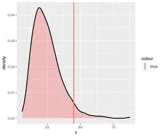
The output of this code gives a distribution and two vertical lines, one red and one blue. But in the legend the blue line is marked "red" and vice versa. What might be the reason? Distribution and 2 vertical lines

variances <- apply(matrix(rexp(40*1000,0.2),1000),1,var) 
hist(variances)
v_theo <- 45 ## need to define v_theo
g <- ggplot(data.frame(x=variances), aes(x = x)) 
g <- g + geom_density(alpha=0.2,size=1,fill="red")
g <- g + geom_vline(aes(xintercept = mean(variances),color="red"), size=1) 
g <- g + geom_vline(aes(xintercept = (v_theo),color="blue"), size=1) 
g
desval
  • 2,345
  • 2
  • 16
  • 23
dhruvak_a
  • 31
  • 7

2 Answers2

1
library(ggplot2)
variances <- apply(matrix(rexp(40*1000,0.2),1000),1,var) 
hist(variances)
v_theo <- 45


g <- ggplot(data.frame(x=variances), aes(x = x)) 
g <- g + geom_density(alpha=0.2,size=1,fill="red")
g <- g + geom_vline(aes(xintercept = v_theo, color="blue"), size=1) 
g

enter image description here

g <- ggplot(data.frame(x=variances), aes(x = x)) 
g <- g + geom_density(alpha=0.2,size=1,fill="red")
g <- g + geom_vline(aes(xintercept = mean(variances),color="mean"), size=1) 
g <- g + geom_vline(aes(xintercept = v_theo,color="v_theo"), size=1) +
  scale_color_manual(name = "Legend name", values = c(mean = "red", v_theo = "blue"))
g

enter image description here

See here as well: Add legend to geom_vline

desval
  • 2,345
  • 2
  • 16
  • 23
0

That's because the colors are mapped by the aes function. If you want to map them manually, you could either take them out of the aes like this

variances <- apply(matrix(rexp(40*1000,0.2),1000),1,var) 
hist(variances)
g <- ggplot(data.frame(x=variances), aes(x = x)) 
g <- g + geom_density(alpha=0.2,size=1,fill="red")
g <- g + geom_vline(aes(xintercept = mean(variances)), color="red", size=1) 
g <- g + geom_vline(aes(xintercept = (v_theo)), color="blue", size=1) 
g

You'll lose the legen by doing this though. If you want the legend, you can use scale_color_manual to fix the order of the colors.

variances <- apply(matrix(rexp(40*1000,0.2),1000),1,var) 
hist(variances)
g <- ggplot(data.frame(x=variances), aes(x = x)) 
g <- g + geom_density(alpha=0.2,size=1,fill="red")
g <- g + geom_vline(aes(xintercept = mean(variances),color="red"), size=1) 
g <- g + geom_vline(aes(xintercept = (v_theo),color="blue"), size=1) 
g <- g + scale_color_manual(values = c("blue", "red"))

g
Sergio Romero
  • 368
  • 1
  • 8