How can I generate an array of numbers between multiple ranges defined in separate cells in Sheet?

Question

A1: 1 | B1: 4
A2: 3 | B2: 6

How can I get {1, 2, 3, 3, 4, 4, 5, 6} out of this?

– – – – – –

I know this way:
=ArrayFormula({ROW(INDIRECT(A1&":"&B1)); ROW(INDIRECT(A2&":"&B2))})

That does the job perfectly but what if I don't know, how many ranges there will be? I want to generate an array of all the numbers between values specified in cells from A1:B1 all the way to A:B.

Thank you in advance!

I provided an answer, but this sounds like an xyproblem.info . If the "numbers" are actually dates, for example, there may be a significantly easier way to manipulate your real data. But you'd need to share a more realistic dataset as well as what the overall goal is rather than just this goal that is a step in a larger goal. — MattKing, Apr 29 '20 at 18:07
Oh, I already asked you a follow up question and only then saw that you commented it here as well. So hear me out. I have columns for every day of a month, then time of when i started working and time when i stopped working, then how much i worked (difference between those times which can pass over midnight). From this I want to know how much I worked in the whole month "in night" (between two specific times). Thanks to you, I've done it. But now, I want the real thing. I want to know how much I worked in night exept the weekends and national holidays. I'm completely out of my league there. — Fakint, Apr 30 '20 at 01:43
Sweet mother of formulas, I've got it. Ca't make it a general formula yet but it works with my sheets. — Fakint, Apr 30 '20 at 10:01
I have a fairly simple way of doing the calculation you're looking for that i think you will be surprised is possible. But i need sample data. you say you have a column for every day of the month a start time and a stop time. If i could just get those 3 columns of data, for a month, as well as what "night" is defined as, i could give you a relatively simple single formula to calculate all the "night" time. — MattKing, Apr 30 '20 at 12:51

score 3 · Answer 1 · answered Apr 29 '20 at 17:56

3

Here is a relatively simple formula to generate the array you're talking about based on an infinite number of ranges in columns A and B.

=ARRAYFORMULA(QUERY(SPLIT(FLATTEN(SEQUENCE(1,MAX(B1:B10-A1:A10)+1,0)+A1:A10&"|"&B1:B10),"|",0,0),"Select Col1 where Col1<=Col2 order by Col1",0))

You can see it demonstrated in the tab called Demo 2 on this sheet.

answered Apr 29 '20 at 17:56

MattKing

7,373
8
13

3

@kishkin This is the disclaimer I use on the Google Help Forums where I am a volunteer "Product Expert": "I should mention that FLATTEN() is an undocumented function that I only recently discovered. I've believe it is intended to remain "hidden" in the back end of the sheets programming, but if what I did is what you're after, there really isn't a more efficient way to do it. If you're uncomfortable using an undocumented function, let me know and I can try to build a different kind of work around for you." – MattKing Apr 29 '20 at 22:32
@Mattking, I can't thank you enough, this is perfect! Althought I must admit, it's completely beyond me how exactly it works. I was playing with it and implemented it to my sheet succesfully, but then lost in it a bit. Would you be so kind and tell me, where exactly would you put some condition in it on the cells from which it generate the ranges? Let's say I want an array from all the values from A1:B, but only if values in C1:C are greater than 10. Is it possible? – Fakint Apr 30 '20 at 01:30
@Fakint could be changed a bit for that: `=ARRAYFORMULA(QUERY(SPLIT(FLATTEN(SEQUENCE(1,MAX(B2:B-A2:A)+1,0)+A2:A&"|"&B2:B&"|"&C2:C),"|",0,0),"Select Col1 where Col1<=Col2 and Col3 > 10 order by Col1",0))` – kishkin Apr 30 '20 at 13:24
@Fakint or this (it will not perform on empty strings): `=ARRAYFORMULA( QUERY( SPLIT( FLATTEN( SEQUENCE( 1, MAX(FILTER(B2:B, A2:A <> "", B2:B <> "", C2:C <> "", C2:C > 10) - FILTER(A2:A, A2:A <> "", B2:B <> "", C2:C > 10)) + 1, 0 ) + FILTER(A2:A, A2:A <> "", B2:B <> "", C2:C > 10) & "|" & FILTER(B2:B, A2:A <> "", B2:B <> "", C2:C > 10) ), "|", 0, 0 ), " Select Col1 where Col1 <= Col2 order by Col1 ", 0 ) )` – kishkin Apr 30 '20 at 13:33

Gary's Student · Answer 2 · 2020-04-29T17:24:12.477

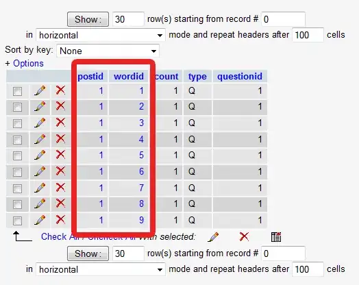
In Excel 365 with your data in columns A and B, pick a cell and enter:

="{" & TEXTJOIN(",",TRUE,SEQUENCE(,MAX(A:B),MIN(A:B))) & "}"

EDIT#1:

Try this VBA macro:

Sub MakeArray()
    Dim I As Long, N As Long, J, k
    Dim strng As String
    Dim arr As Variant

    N = Cells(Rows.Count, "A").End(xlUp).Row
    For I = 1 To N
        For J = Cells(I, 1) To Cells(I, 2)
            strng = strng & "," & J
        Next J
    Next I
    strng = Mid(strng, 2)

    strng = "{" & Join(fSort(Split(strng, ",")), ",") & "}"


    MsgBox strng
End Sub

Public Function fSort(ByVal arry)
Dim I As Long, J As Long, Low As Long
    Dim Hi As Long, Temp As Variant

    Low = LBound(arry)
    Hi = UBound(arry)

    J = (Hi - Low + 1) \ 2
    Do While J > 0
        For I = Low To Hi - J
          If arry(I) > arry(I + J) Then
            Temp = arry(I)
            arry(I) = arry(I + J)
            arry(I + J) = Temp
          End If
        Next I
        For I = Hi - J To Low Step -1
          If arry(I) > arry(I + J) Then
            Temp = arry(I)
            arry(I) = arry(I + J)
            arry(I + J) = Temp
          End If
        Next I
        J = J \ 2
    Loop
    fSort = arry
End Function

The macro:

creates a comma-separated string from each A/B pair
sorts the string
outputs the string

Thank you, but Ineed all the values, not just range from MIN and MAX. This generates {1, 2, 3, 4, 5, 6} but I need {1, 2, 3, 3, 4, 4, 5, 6} with all the duplicites (I work with them later). — Fakint, Apr 29 '20 at 16:04

How can I generate an array of numbers between multiple ranges defined in separate cells in Sheet?

2 Answers2

Linked