Python: fitting curve to masked data with scipy curve_fit

Question

I'm trying to write a script with python/numpy/scipy for data manipulation, fitting and plotting of angle dependent magnetoresistance measurements. I'm new to Python, got the frame code from my PhD advisor, and managed to add few hundred lines of code to the frame. After a while I noticed that some measurements had multiple blunders, and since the script should do all the manipulation automatically, I tried to mask those points and fit the curve to the unmasked points (the curve is a sine squared superposed on a linear function, so numpy.ma.polyfit isn't really a choice). However, after masking both x and y coordinates of the problematic points, the fitting would still take them into consideration, even though they wouldn't be shown in the plot. The example is simplified, but the same is happening;

import numpy.ma as ma
import matplotlib.pyplot as plt
from scipy.optimize import curve_fit



def Funk(x, k, y0):
 return k*x + y0   

fig,ax= plt.subplots()

x=ma.masked_array([1,2,3,4,5,6,7,8,9,10],mask=[0,0,0,0,0,0,1,1,1,1])
y=ma.masked_array([1,2,3,4,5,30,35,40,45,50], mask=[0,0,0,0,0,1,1,1,1,1])


fitParamsFunk, fitCovariancesFunk = curve_fit(Funk, x, y)

ax.plot(x, Funk(x, fitParamsFunk[0], fitParamsFunk[1]))
ax.errorbar(x, y, yerr = None, ms=3, fmt='-o')
plt.show()

The second half of the points is masked and not shown in the plot, but still taken into consideration.

While writing the post I figured out that I can do this:

def Funk(x, k, y0):
    return k*x + y0   

fig,ax= plt.subplots()

x=np.array([1,2,3,4,5,6,7,8,9,10])
y=np.array([1,2,3,4,5,30,35,40,45,50])
mask=np.array([0,0,0,0,0,1,1,1,1,1])

fitParamsFunk, fitCovariancesFunk = curve_fit(Funk, x[mask], y[mask])

ax.plot(x, Funk(x, fitParamsFunk[0], fitParamsFunk[1]))
ax.errorbar(x, y, yerr = None, ms=3, fmt='-o')
plt.show()

What I actually wanted

I guess that scipy curve_fit isn't meant to deal with masked arrays, but I still would like to know whether there is any workaround for this (I need to work with masked arrays because the number of data points is >10e6, but I'm only plotting 100 at once, so I would need to take the mask of the part of the array that I want to plot and assign it to another array, while copying the values of the array to another or setting the original mask to False)? Thanks for any suggestions

Answer 1

If you only want to consider the valid entries, you can use the inverse of the mask as an index:

x = ma.masked_array([1,2,3,4,5,6,7,8,9,10], mask=[0,0,0,0,0,1,1,1,1,1])  # changed mask
y = ma.masked_array([1,2,3,4,5,30,35,40,45,50], mask=[0,0,0,0,0,1,1,1,1,1])

fitParamsFunk, fitCovariancesFunk = curve_fit(Funk, x[~x.mask], y[~y.mask])

PS: Note that both arrays need to have the same amount of valid entries.

Answer 2

I think that what you want to do is to define a mask that lists the indices of the "good data points" and then use that as the points to fit (and/or to plot).

As a lead author of lmfit, I would recommend using that library for curve-fitting: it has many useful features over curve_fit. With this, your example might look like this:

import numpy as np
import matplotlib.pyplot as plt
from lmfit import Model

def Funk(x, k, y0, good_points=None):  # note: add keyword argument
    f = k*x + y0
    if good_points is not None:
        f = f[good_points]       # apply mask of good data points
    return f

x = np.array([1,2,3,4,5, 6,7,8.,9,10])
y = np.array([1,2,3,4,5,30,35.,40,45,50]) 
y += np.random.normal(size=len(x), scale=0.19) # add some noise to make it fun

# make an array of the indices of the "good data points"
# does not need to be contiguous.
good_points=np.array([0,1,2,3,4])

# turn your model function Funk into an lmfit Model
mymodel = Model(Funk)

# create parameters, giving initial values. Note that parameters are
# named using the names of your function's argument and that keyword 
# arguments with non-numeric defaults like 'good points' are seen to
#  *not* be parameters. Like the independent variable `x`, you'll 
# need to pass that in when you do the fit.
# also: parameters can be fixed, or given `min` and `max` attributes

params = mymodel.make_params(k=1.4,  y0=0.2)
params['k'].min = 0

# do the fit to the 'good data', passing in the parameters, the 
# independent variable `x` and the `good_points` mask.
result  = mymodel.fit(y[good_points], params, x=x, good_points=good_points)

# print out a report of best fit values, uncertainties, correlations, etc.
print(result.fit_report())

# plot the results, again using the good_points array as needed.
plt.plot(x, y, 'o', label='all data')
plt.plot(x[good_points], result.best_fit[good_points], label='fit to good data')
plt.legend()
plt.show()

This will print out

[[Model]]
    Model(Funk)
[[Fit Statistics]]
    # fitting method   = leastsq
    # function evals   = 7
    # data points      = 5
    # variables        = 2
    chi-square         = 0.02302999
    reduced chi-square = 0.00767666
    Akaike info crit   = -22.9019787
    Bayesian info crit = -23.6831029
[[Variables]]
    k:   1.02460577 +/- 0.02770680 (2.70%) (init = 1.4)
    y0: -0.04135096 +/- 0.09189305 (222.23%) (init = 0.2)
[[Correlations]] (unreported correlations are < 0.100)
    C(k, y0) = -0.905

and produce a plot of

hope that helps get you started.

Answer 3

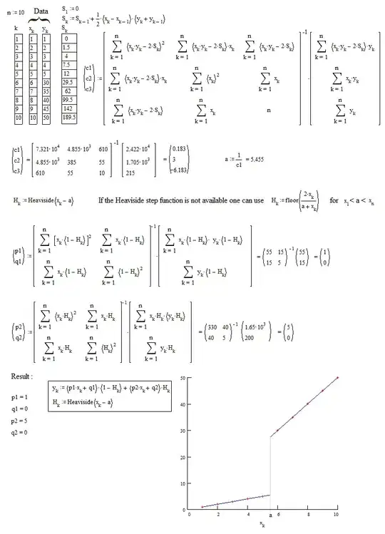
The use of mask in numerical calculus is equivalent to the use of the Heaviside step function in analytical calculus. For example this becomes very simple by application for piecewise linear regression:

They are several examples of piecewise linear regression in the paper : https://fr.scribd.com/document/380941024/Regression-par-morceaux-Piecewise-Regression-pdf

Using the method shown in this paper, the very simple calculus below leads to the expected form of result :

Note : In case of large number of points, if there was several points with slightly different abscissae in the transition area it sould be more accurate to apply the case considered pages 29-31 of the paper referenced above.