How to resize of bins/pixels when zooming

Question

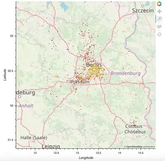
I am currently trying to project a dataset (Berlin public transport spots) on to map tiles with the help of datashader and bokeh. To certain extents it worked nicely, while three problems remain:

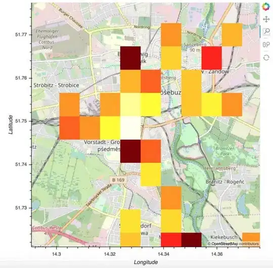
1. when zooming into the data, the pixels remain rather large and are not rearranged - how to do this?
2. how to get the projected data semi-transparent to still see the map below?
3. the "save"-function of the bokeh toolbar disappeared, as the map tiles were merged. How to get it back?

Thanks for any input!

the (far from perfect) code written:

import numpy as np
import pandas as pd
import geopandas as gp
import datashader as ds
import datashader.transfer_functions as tf
from datashader.utils import export_image
from datashader.utils import lnglat_to_meters as webm
from datashader.colors import Hot
import dask.dataframe as dd
import multiprocessing as mp
from functools import partial
from IPython.core.display import HTML, display
import matplotlib.pyplot as plt
import holoviews as hv
from holoviews.operation.datashader import datashade, dynspread
hv.extension("bokeh", "matplotlib")
from bokeh.io import output_file, output_notebook, show
from bokeh.plotting import figure, show
from holoviews import dim, opts
import geoviews as gv
from colorcet import palette, fire

#get official data of bus/subway stops in Berlin
# -> https://www.vbb.de/media/download/2035
#read data
df = pd.read_csv('UMBW.CSV', engine= 'python', sep=';', usecols=['Y-Koordinate', 'X-Koordinate'])

##some formatting
##replace comma by point
df = df.apply(lambda x: x.str.replace(',','.'))
#delete rows witn NaN -> pandas.DataFrame.dropna
df = df.dropna()
#entries were objects - need to convert to floats
df['X-Koordinate']=pd.to_numeric(df['X-Koordinate'])
df['Y-Koordinate']=pd.to_numeric(df['Y-Koordinate'])

# Project longitude and latitude onto web mercator plane.
df.loc[:, 'easting'], df.loc[:, 'northing'] = webm(df['X-Koordinate'],df['Y-Koordinate'])

# Getting range/box of latitude and longitude for plotting later.
# drop the points lying on the border
y_range_min = df['Y-Koordinate'].quantile(0.01)
y_range_max = df['Y-Koordinate'].quantile(0.99)
x_range_min = df['X-Koordinate'].quantile(0.01)
x_range_max = df['X-Koordinate'].quantile(0.99)

#cornerspots for canvas
sw = webm(x_range_min,y_range_min)#southwest
ne = webm(x_range_max,y_range_max)#northeast
SF = zip(sw, ne)

dask_df = dd.from_pandas(df, npartitions=mp.cpu_count())
dask_df = dask_df.compute()

display(HTML("<style>.container { width:100% !important; }</style>"))

plot_width = int(3600)
plot_height = int(3600)
cvs = ds.Canvas(plot_width, plot_height, *SF)
agg = cvs.points(dask_df, 'easting', 'northing')

#dynamic map tiles -> https://wiki.openstreetmap.org/wiki/Tile_servers
#url="http://server.arcgisonline.com/ArcGIS/rest/services/World_Imagery/MapServer/tile/{Z}/{Y}/{X}.png"
url="https://a.tile.openstreetmap.org/{Z}/{X}/{Y}.png"
geomap = gv.WMTS(url)

#manipulate pixelsize for zoom
dynspread.max_px=1
dynspread.threshold=0.1

points = hv.Points(gv.Dataset(dask_df, kdims=['easting', 'northing']))
bvg_stops = dynspread(datashade(points, cmap=Hot).opts(height=640,width=640))
fig = geomap * bvg_stops
hv.save(fig, 'berlin.html', backend='bokeh')

An example output of the initial bokeh plot and a zoomed in version (around the city of Cottbus).

Answer 1

1. "when zooming into the data, the pixels remain rather large and are not rearranged - how to do this?"

   Datashader is a Python program that produces an array of rasterized values when given a data structure. Here, it is rendering your data as requested, and you are then saving the output of it to an HTML file using hv.save. Once you do that you will have a figure that will never update. You'll zoom in on the HTML page, causing the browser's JavaScript code to request an update from Python, but Python is not running and cannot respond to the request for an updated figure. If you want a zoomable image exported to HTML, you'll need to either specify a much higher initial resolution with something like datashade(..., dynamic=False, height=4000, width=4000) (which will give a big file size and may not look great initially, but will allow some degree of zooming), or else generate a whole set of data tiles at lots of various resolutions (supported by Datashader but not yet well documented), or else (for full power) use Bokeh server to provide a Python process to accompany the HTML/JavaScript code. I.e., either generate a bit more data initially, generate all combinations of data beforehand, or provide a server that can regenerate them on demand. Without one of those approaches, you should not expect to have any data available beyond the initial rendering.

2. how to get the projected data semi-transparent to still see the map below?

   bvg_stops.opts(alpha=0.5). You can also consider using Panel.pyviz.org to add some widgets for opacity for the map and the data to let you turn them on and off interactively; see examples.pyviz.org for examples.

3. the "save"-function of the bokeh toolbar disappeared, as the map tiles were merged. How to get it back?

   Unfortunately, this is a limitation caused by the browser's security model, and is not something Bokeh or any of the other tools here can override. The map tiles come from a separate server, and browsers disable exporting such "cross-origin" content to avoid certain security issues (Can't Save Bokeh Plot with Panel from PyViz Example).