Sine curve fit using lm, nls and nls2 in R

Question

I acquired data (motor adaptation =y in function of delays =t ) which I expect to look like a sine wave. I am trying to:

Fit a sine curve in my data
Estimate the best model/parameters.

I have read several posts here, here and here but I am still struggling.

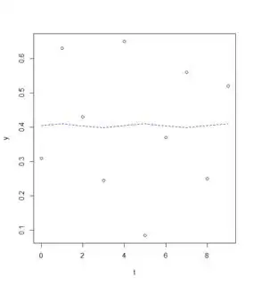
1) Using lm

Code:

t<-c(0, 1, 2, 3, 4, 5, 6, 7, 8, 9)
y<-c(0.310 ,0.630 ,0.430 ,0.245, 0.650 ,0.085 ,0.370, 0.560 ,0.250, 0.520)
reslm <- lm(y ~ sin(pi/2*t)+ cos(pi/2*t)) #my period is supposed to be 4, so period equals to pi/2
summary(reslm)
rg<-(max(y)-min(y)/2)
plot(y~t)
lines(fitted(reslm)~t,col=4,lty=2)

Output:

lm(formula = y ~ sin(pi/2 * t) + cos(pi/2 * t))

Residuals:
     Min       1Q   Median       3Q      Max 
-0.32450 -0.13956 -0.00325  0.14819  0.24450 

Coefficients:
              Estimate Std. Error t value Pr(>|t|)    
(Intercept)   0.404375   0.067993   5.947 0.000572 ***
sin(pi/2 * t) 0.005125   0.095190   0.054 0.958567    
cos(pi/2 * t) 0.001125   0.095190   0.012 0.990900    
---
Signif. codes:  0 ‘***’ 0.001 ‘**’ 0.01 ‘*’ 0.05 ‘.’ 0.1 ‘ ’ 1

Residual standard error: 0.2107 on 7 degrees of freedom
Multiple R-squared:  0.0004303, Adjusted R-squared:  -0.2852 
F-statistic: 0.001507 on 2 and 7 DF,  p-value: 0.998

Graph:

Questions:

I am super confused, how can I change the amplitude as well as the phase shift?
How can I improve my fit using this methods?

2) Using nls

I used the equation y(t) = A*sin(Omega*t + Phi) + C where A is the amplitude, Omega the period, Phi the phase shift and C the midline.

Code:

t<-c(0, 1, 2, 3, 4, 5, 6, 7, 8, 9)
y<-c(0.310 ,0.630 ,0.430 ,0.245, 0.650 ,0.085 ,0.370, 0.560 ,0.250, 0.520)

A<- (max(y)-min(y)/2)
C<-((max(y)+min(y))/2)

res1<- nls(y ~ A*sin(omega*t+phi)+C, data=data.frame(t,y), start=list(A=A,omega=pi/2,phi=0,C=C))
summary(res1)
co <- coef(res1)
resid(res1)
sum(resid(res1)^2)
fit <- function(x, a, b, c, d) {a*sin(b*x+c)+d}
# Plot result
plot(x=t, y=y)
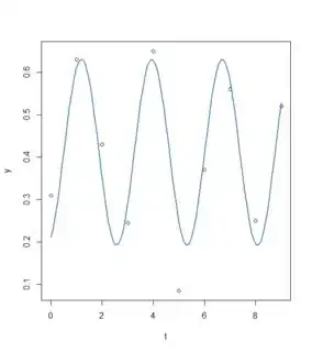
curve(fit(x, a=co["A"], b=co["omega"], c=co["phi"], d=co["C"]), add=TRUE ,lwd=2, col="steelblue")

Output:

Formula: y ~ A * sin(omega * t + phi) + C

Parameters:
       Estimate Std. Error t value Pr(>|t|)    
A       0.21956    0.03982   5.513   0.0015 ** 
omega   2.28525    0.07410  30.841 7.72e-08 ***
phi   -32.57364    0.40375 -80.678 2.44e-10 ***
C       0.41146    0.02926  14.061 8.07e-06 ***
---
Signif. codes:  0 ‘***’ 0.001 ‘**’ 0.01 ‘*’ 0.05 ‘.’ 0.1 ‘ ’ 1

Residual standard error: 0.09145 on 6 degrees of freedom

Number of iterations to convergence: 18 
Achieved convergence tolerance: 9.705e-06

Graph:

Questions:

This methods seem to work a bit better, but how can I improve the fit using this method? I tried to change some parameters manually, for example, changing the phase shift (phi) does not do much or lead to an error (see part 3).

3) Using nls and nsl2, in order to tune my model

Code:

###nls2
t<-c(0, 1, 2, 3, 4, 5, 6, 7, 8, 9)
y<-c(0.310 ,0.630 ,0.430 ,0.245, 0.650 ,0.085 ,0.370, 0.560 ,0.250, 0.520)
A <- (max(y)-min(y)/2)
C<-((max(y)+min(y))/2)
pp <- expand.grid(omega=(c(2.094395, 1.570796,  1.256637)), phi=(-1:1), A=A, C=C) # omega = 2*pi/3, pi/2 , 2*pi/5
View(pp)
pp1<-data.frame(pp)
res2<- nls2(y ~ A*sin(omega*t+phi)+C, data=data.frame(t,y), start=pp1,  algorithm = "brute-force")
res2
summary(res2)
co <- coef(res2)
resid(res2)
sum(resid(res2)^2)
fit <- function(x, a, b, c, d) {a*sin(b*x+c)+d}
# Plot result 
plot(x=t, y=y)
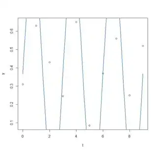
curve(fit(x, a=co["A"], b=co["omega"], c=co["phi"], d=co["C"]), add=TRUE ,lwd=2, col="steelblue")

#optimisation
res3<-nls2(y ~ A*sin(omega*t+phi)+C, start = res2)
res3
summary(res3)
co3 <- coef(res3)
resid(res3)
sum(resid(res3)^2)
fit <- function(x, a, b, c, d) {a*sin(b*x+c)+d}
# Plot result
plot(x=t, y=y)
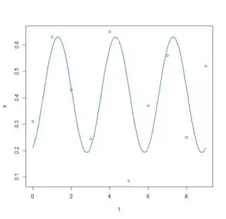
curve(fit(x, a=co3["A"], b=co["omega"], c=co3["phi"], d=co3["C"]), add=TRUE ,lwd=2, col="steelblue")

Output:

First attempt (nls2 model1):

model: y ~ A * sin(omega * t + phi) + C
   data: data.frame(t, y)
 omega    phi      A      C 
2.0944 0.0000 0.6075 0.3675 
 residual sum-of-squares: 0.8545

Number of iterations to convergence: 9 
Achieved convergence tolerance: NA
> summary(res2)

Formula: y ~ A * sin(omega * t + phi) + C

Parameters:
      Estimate Std. Error t value Pr(>|t|)    
omega  2.09440    0.08453  24.776 2.84e-07 ***
phi    0.00000    0.46494   0.000   1.0000    
A      0.60750    0.17851   3.403   0.0144 *  
C      0.36750    0.12044   3.051   0.0225 *  
---
Signif. codes:  0 ‘***’ 0.001 ‘**’ 0.01 ‘*’ 0.05 ‘.’ 0.1 ‘ ’ 1

Residual standard error: 0.3774 on 6 degrees of freedom

Number of iterations to convergence: 9 
Achieved convergence tolerance: NA

Graph:

Second attempt (nls2 model2):

Nonlinear regression model
  model: y ~ A * sin(omega * t + phi) + C
   data: <environment>
  omega     phi       A       C 
 2.2852 -1.1577  0.2196  0.4115 
 residual sum-of-squares: 0.05018

Number of iterations to convergence: 12 
Achieved convergence tolerance: 8.075e-06
> summary(res3)

Formula: y ~ A * sin(omega * t + phi) + C

Parameters:
      Estimate Std. Error t value Pr(>|t|)    
omega  2.28524    0.07410  30.841 7.72e-08 ***
phi   -1.15769    0.40375  -2.867   0.0285 *  
A      0.21956    0.03982   5.513   0.0015 ** 
C      0.41146    0.02926  14.061 8.07e-06 ***
---
Signif. codes:  0 ‘***’ 0.001 ‘**’ 0.01 ‘*’ 0.05 ‘.’ 0.1 ‘ ’ 1

Residual standard error: 0.09145 on 6 degrees of freedom

Number of iterations to convergence: 12 
Achieved convergence tolerance: 8.075e-06

Graph:

Questions:

So here it seems I misunderstood what nls2 was doing as I am finding exactly the same results as part 2. I still do not know which parameters are the best, how can I do this?

4) Using nls, in order to tune my model by looping through several parameters

Code:

t<-c(0, 1, 2, 3, 4, 5, 6, 7, 8, 9)
y<-c(0.310 ,0.630 ,0.430 ,0.245, 0.650 ,0.085 ,0.370, 0.560 ,0.250, 0.520)
A <- (max(y)-min(y)/2)
C<-((max(y)+min(y))/2)
pp <- expand.grid(omega=(c(2.094395, 1.570796,  1.256637)), phi=(-1:1), A=A, C=C) # omega = 2*pi/3, pi/2 , 2*pi/5
#View(pp)

fit_AIC<- vector()
fit_BIC<- vector()

coef_A<- vector()
coef_ome<- vector()
coef_phi<- vector()
coef_C<- vector()
RSS<-vector()

for (ii in 1:nrow(pp))
{
    res<- nls(y ~ A*sin(omega*t+phi)+C, data=data.frame(t,y), start=list(A=pp$A[ii],omega=pp$omega[ii],phi=pp$phi[ii],C=pp$C[ii]), trace = TRUE)
    fit_AIC[ii]<-AIC(res)
    fit_BIC[ii]<-BIC(res)

    coef_A[ii]<- coef(res)[1]
    coef_ome[ii]<- coef(res)[2]
    coef_phi[ii]<- coef(res)[3]
    coef_C[ii]<- coef(res)[4]
    RSS<-sum(resid(res)^2)

}

results<-data.frame(RSS, fit_AIC,  fit_BIC,  coef_A,  coef_ome,  coef_phi,  coef_C)
View(results)

Output:

I get this error:

1.405742 :   0.607500  2.094395 -1.000000  0.367500
0.1448148 :   0.1563179  2.1441802 -0.9937729  0.4172079

...


0.05018035 :   0.2195573  2.2852482 -1.1577097  0.4114573
2.085664 :  0.607500 1.570796 1.000000 0.367500
0.3104012 :  0.01321257 1.60518024 0.83201816 0.40437498
0.3098916 :   0.0180852  3.0888764 -5.9933691  0.4060743
Error in nls(y ~ A * sin(omega * t + phi) + C, data = data.frame(t, y),  : 
  le pas 0.000488281 est devenu inférieur à 'minFactor' de 0.000976562


        RSS    fit_AIC    fit_BIC     coef_A  coef_ome    coef_phi    coef_C
1 0.05018035 -14.568398 -13.055473 0.21955754 2.2852455  -1.1576955 0.4114573
2 0.05018035   2.753153   4.266079 0.07487110 0.8575642   0.2299909 0.3916769
3 0.05018035   2.753153   4.266079 0.07487109 0.8575736   0.2299951 0.3916763
4 0.05018035 -14.568398 -13.055473 0.21955763 2.2852443  -1.1576894 0.4114573
5 0.05018035 -14.568398 -13.055473 0.21955729 2.2852490 -32.5736406 0.4114573
6 0.05018035   2.753153   4.266079 0.07487105 0.8575619   0.2300021 0.3916770
7 0.05018035 -14.568398 -13.055473 0.21955735 2.2852482  -1.1577097 0.4114573

Questions:

So this error seems to be because my initial parameters are wrong. Is this correct? But how can I estimate the best parameters if the majority of parameters do not work?
Also, I do not understand why the RSS is always the same despite different parameters
And why do I observe only 2 different AIC and 2 different BIC while the models are different?

Any kind of help would be much appreciated, thanks.

You are minimizing the same function in all rows of the table at the end and that function has multiple local minima. For example, look at this graph: `curve(x^4 - 4 * x^3 - 2 * x^2 + 9 * x + 9, -2, 5)`. If you minimize that function with a starting value near the left of the graph you would likely get the first local minimum and if you started with a starting value near the right you would likely get the second. — G. Grothendieck, Jan 10 '20 at 17:23
Hello, thanks for your reply but I am a bit confused. To which of my questions are you replying here ? And what should I do to find the best parameters? Or should I accept results of point 2) as my best fit? Thanks — SophieB, Jan 15 '20 at 12:18

score 1 · Answer 1 · answered Jan 11 '20 at 00:29

On the first model you're effectiveluy fitting the model y = A*sin(pi/2 * t) + B*cos(pi/2 * t) + C and you can't change the phase shift with that approach. On the next steps you can fit an appropiated equation. nls performs a non linear regresion with the provided model and nls2 adds an extra step by creating a grid of initial parameters and performing several nls calls. And in the last approach you coded a similar strategy as nls2. But some initial conditions lead to an error.

The objetive function that you minimize have multiple local minima, just like in the example the function have multiple minima with different coordinates.

Also when you change the equation to y ~ A * sin(omega * t + phi) + C you have four parameters to be determinated and only nine data points you need to add more data points to get a better estimation of the parameters. You can also normalize the data to 0-1 range.

Hope it helps

score 1 · Answer 2 · edited Sep 24 '21 at 09:56

Using lm: Your period is ~2.75 instead of 4.

  t<-c(0, 1, 2, 3, 4, 5, 6, 7, 8, 9)
  y<-c(0.310 ,0.630 ,0.430 ,0.245, 0.650 ,0.085 ,0.370, 0.560 ,0.250, 0.520)

  reslm <- lm(y ~ cos(2* pi/2.75*t) + sin(2* pi/2.75*t))

  summary(reslm)

  coef1 <- coef(reslm)

  plot(y~t)

  t1 <- seq(0,9,.1)
  y1 <- coef1[2] * cos(2*pi/2.75*t1) + coef1[3] * sin(2* pi/2.75*t1) + coef1[1]

  lines(t1,y1,col=2)

Sine curve fit using lm, nls and nls2 in R

1) Using lm

2) Using nls

3) Using nls and nsl2, in order to tune my model

4) Using nls, in order to tune my model by looping through several parameters

2 Answers2