12

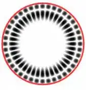
I am looking to plot something like the whispering gallery modes -- a 2D cylindrically symmetric plot in polar coordinates. Something like this:

whispering gallery modes

I found the following code snippet in Trott's symbolics guidebook. Tried running it on a very small data set; it ate 4 GB of memory and hosed my kernel:

(* add points to get smooth curves *)
addPoints[lp_][points_, \[Delta]\[CurlyEpsilon]_] := 
Module[{n, l}, Join @@ (Function[pair,
       If[(* additional points needed? *)
          (l = Sqrt[#. #]&[Subtract @@ pair]) < \[Delta]\[CurlyEpsilon], pair, 
          n = Floor[l/\[Delta]\[CurlyEpsilon]] + 1; 
          Table[# + i/n (#2 - #1), {i, 0, n - 1}]& @@ pair]] /@ 
          Partition[If[lp === Polygon, 
                       Append[#, First[#]], #]&[points], 2, 1])]

(* Make the plot circular *)
With[{\[Delta]\[CurlyEpsilon] = 0.1, R = 10}, 
 Show[{gr /. (lp : (Polygon | Line))[l_] :> 
     lp[{#2 Cos[#1], #2 Sin[#1]} & @@@(* add points *)
       addPoints[lp][l, \[Delta]\[CurlyEpsilon]]], 
   Graphics[{Thickness[0.01], GrayLevel[0], Circle[{0, 0}, R]}]}, 
  DisplayFunction -> $DisplayFunction, Frame -> False]]

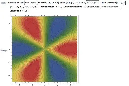
Here, gr is a rectangular 2D ListContourPlot, generated using something like this (for example):

data = With[{eth = 2, er = 2, wc = 1, m = 4}, 
   Table[Re[
     BesselJ[(Sqrt[eth] m)/Sqrt[er], Sqrt[eth] r wc] Exp[
       I m phi]], {r, 0, 10, .2}, {phi, 0, 2 Pi, 0.1}]];
gr = ListContourPlot[data, Contours -> 50, ContourLines -> False, 
  DataRange -> {{0, 2 Pi}, {0, 10}}, DisplayFunction -> Identity, 
  ContourStyle -> {Thickness[0.002]}, PlotRange -> All, 
  ColorFunctionScaling -> False]

Is there a straightforward way to do cylindrical plots like this?.. I find it hard to believe that I would have to turn to Matlab for my curvilinear coordinate needs :)

Leo Alekseyev
  • 12,893
  • 5
  • 44
  • 44
  • Since you preferred the analytical solution instead of the numerical solution, i.e. `ContourPlot` v. `ListContourPlot`, you should change the title to reflect the fact. – rcollyer Apr 24 '11 at 22:57

2 Answers2

12

Previous snippets deleted, since this is clearly the best answer I came up with:

With[{eth = 2, er = 2, wc = 1, m = 4}, 
 ContourPlot[
  Re[BesselJ[(Sqrt[eth] m)/Sqrt[er], Sqrt[eth] r wc] Exp[I phi m]]/. 
                                         {r ->Norm[{x, y}], phi ->ArcTan[x, y]}, 
  {x, -10, 10}, {y, -10, 10}, 
  Contours -> 50, ContourLines -> False, 
  RegionFunction -> (#1^2 + #2^2 < 100 &), 
  ColorFunction -> "SunsetColors"
 ]
]

enter image description here

Edit

Replacing ContourPlot by Plot3D and removing the unsupported options you get:

enter image description here

Dr. belisarius
  • 60,527
  • 15
  • 115
  • 190
  • @belisarius I changed DensityPlot to ContourPlot since it runs _much_ faster for me and produces similar results. Either one works fine. – Leo Alekseyev Apr 24 '11 at 07:42
  • @belisarius, I'd wrap the `Replace` with `Evaluate` to avoid the problems you get with `Plot` when you don't. – rcollyer Apr 25 '11 at 03:32
  • @rcollyer I already read that comment in your answer, and I think it is right. But in this case it seems not necessary. I really did not think much about it, but if you understand there is a hidden potential problem there, feel free to edit my code. An explanation about when it is needed, and when not would be great too. – Dr. belisarius Apr 25 '11 at 03:38
  • @belisarius, good question. I'm never sure myself, although `Plot` itself seems to be the worst offender. – rcollyer Apr 25 '11 at 03:58
7

This is a relatively straightforward problem. The key is that if you can parametrize it, you can plot it. According to the documentation both ListContourPlot and ListDensityPlot accept data in two forms: an array of height values or a list of coordinates plus function value ({{x, y, f} ..}). The second form is easier to deal with, such that even if your data is in the first form, we'll transform it into the second form.

Simply, to transform data of the form {{r, t, f} ..} into data of the form {{x, y, f} ..} you doN[{#[[1]] Cos[ #[[2]] ], #[[1]] Sin[ #[[2]] ], #[[3]]}]& /@ data, when applied to data taken from BesselJ[1, r/2] Cos[3 t] you get

code for and plot of numerical data

What about when you just have an array of data, like this guy? In that case, you have a 2D array where each point in the array has known location, and in order to plot it, you have to turn it into the second form. I'm partial to MapIndexed, but there are other ways of doing it. Let's say your data is stored in an array where the rows correspond to the radial coordinate and the columns are the angular coordinate. Then to transform it, I'd use

R = 0.01;    (*radial increment*)
T = 0.05 Pi; (*angular increment*)
xformed = MapIndexed[ 
   With[{r = #2[[1]]*R, t = #2[[1]]*t, f = #1},
   {r Cos[t], r Sin[t], f}]&, data, {2}]//Flatten[#,1]&

which gives the same result.


If you have an analytic solution, then you need to transform it to Cartesian coordinates, like above, but you use replacement rules, instead. For instance,

ContourPlot[ Evaluate[
    BesselJ[1, r/2]*Cos[3 t ] /. {r -> Sqrt[x^2 + y^2], t -> ArcTan[x, y]}], 
   {x, -5, 5}, {y, -5, 5}, PlotPoints -> 50, 
   ColorFunction -> ColorData["DarkRainbow"], Contours -> 25]

gives

analytic plot of Bessel in cylindrical coordinates

Two things to note: 1) Evaluate is needed to ensure that the replacement is performed correctly, and 2) ArcTan[x, y] takes into account the quadrant that the point {x,y} is found in.

Community
  • 1
  • 1
rcollyer
  • 10,475
  • 4
  • 48
  • 75
  • The data could be generated via `data = With[{eth = 2, er = 2, wc = 1, m = 4}, Flatten[#, 1] &@ Table[{r, phi, Re[BesselJ[(Sqrt[eth] m)/Sqrt[er], Sqrt[eth] r wc] Exp[ I m phi]]}, {r, 0, 10, .15}, {phi, 0, 2 Pi, 0.035}]]` This is a reasonable way to go and gives you lots of control, but isn't as concise as belisarius's final answer :) – Leo Alekseyev Apr 24 '11 at 07:52