Complex PDE (Ginzburg Landau) in Julia with Pseudo-Spectral method

Question

I want to teach myself about solving PDEs with Julia and I am trying to solve the complex Ginzburg Landau equation (CGLE) with a pseudospectral method in Julia now. However, I struggle with it and I am a bit of ideas what to try.

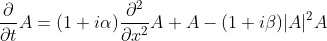
The CGLE reads:

With Fourier transform and its inverse , I can transform into the spectral form:

This is for example also given in this old script I found (https://www.uni-muenster.de/Physik.TP/archive/fileadmin/lehre/NumMethoden/SoSe2009/Skript/script.pdf) From the same source I know, that alpha=1, beta=2 and initial conditions with small noise of order 0.01 around 0 should result in plane waves as solutions. Thats what I want to test first.

Following the very nice tutorial from Chris Rackauckas (https://youtu.be/okGybBmihOE), I tried to use ApproxFun and DifferentialEquations in the following way to solve this problem:

EDIT: I corrected two mistakes from the original post, a missing dot and minus sign, but the code is still not giving the correct results

EDIT2: Figured out that I computed the wavenumber k completely wrong

using ApproxFun
using DifferentialEquations

F = Fourier()
n = 512
L = 100
T = ApproxFun.plan_transform(F, n)
Ti = ApproxFun.plan_itransform(F, n)
x = collect(range(-L/2,stop=L/2, length=n))
k = points(F, n)

alpha = 1im
beta = 2im
u0 = 0.01*(rand(ComplexF64, n) .- 0.5)
Fu0 = T*u0

function cgle!(du, u, p, t)
    a, b, k, T, Ti = p

    invu = Ti*u
    du .= (1.0 .- k.^2*(1.0 .+a)).*u .- T*( (1.0 .+b) .* (abs.(invu)).^2 .* invu)
end

pars = alpha, beta, k, T, Ti
prob = ODEProblem(cgle!, Fu0, (0.,50.), pars)
u = solve(prob, Rodas5(autodiff=false))

# plotting on a equidistant time stepping
t = collect(range(0, stop=50, length=1000))
sol = zeros(eltype(u),(n, length(t)))
for it in eachindex(t)
   sol[:,it] = Ti*u(t[it])
end

IM = PyPlot.imshow(real.(sol))
cb = PyPlot.colorbar(IM, orientation="horizontal")
gcf()

(edited) I tried different solvers, as also recommended in the video, some apparently wont work for complex numbers, some do, but when I run this code it does not give the expected results. The solution remain very small in value and it wont result in the plane waves that actually should be the result. I also tested other intial conditions that should result in chaos, but those result in the same very small solutions as well. I also alternativly used an explicit Laplace Operator with ApproxFun, but the results are the same. My problem here, is that I am neither really an expert with PDE mathemitacaly, nor with their numerical treatment, so far I mainly worked with ODEs.

EDIT2 This now seems to work more or less. I am still wondering about some things though

• How can I compute this on a specified domain like , I am seriously confused about how this works with ApproxFun, as far as I can see the wavenumbers k should be (2pi/L)*[-N/2+1 ; N/2 -1], but I am not so sure about how to do this with ApproxFun
• https://codeinthehole.com/tutorial/coherent.html shows the different dynamic regimes / phase portrait of the equation. While I can reproduce some of them, some don't seem to work, like the Spatio-temporal intermittency

EDIT 3: I solved these issues by using FFTW directly instead of ApproxFun. In case somebody knows how to this with ApproxFun, I would still be interessted though. Below follows the code with FFTW (it is also a bit more optimized for performance)

begin
   using FFTW
   using DifferentialEquations
   using PyPlot
end

begin
   n = 512
   L = 200
   n2 = Int(n/2)
   alpha = 2im
   beta = 1im
   x = range(-L/2,stop=L/2,length=n)
   u0 = 0.01*(rand(ComplexF64, n) .- 0.5)

   k = [0:n/2-1; 0; -n/2+1:-1] .*(2*pi/L);
   k2 = k.*k
   k2[n2 + 1] = (n2*(2*pi/L))^2 

   T = plan_fft(u0)
   Ti = plan_ifft(T*u0)

   LinOp = (1.0 .- k2.*(1.0 .+alpha))
   Fu0 = T*u0
end

function cgle!(du, u, p, t)
    LinOp, b, T, Ti = p

    invu = Ti*u
    du .= LinOp.*u .- T*( (1.0 .+b) .* (abs.(invu)).^2 .* invu)
end

pars = LinOp, beta, T, Ti
prob = ODEProblem(cgle!, Fu0, (0.,100.), pars)
@time u = solve(prob)

t = collect(range(0, stop=50, length=1000))
sol = zeros(eltype(u),(n, length(t)))
for it in eachindex(t)
   sol[:,it] = Ti*u(t[it])
end

IM = PyPlot.imshow(abs.(sol))
cb = PyPlot.colorbar(IM, orientation="horizontal") 
gcf()

EDIT 4: Rodas turned out to be a extremly slow solver for this case, just using the default works out nicely for me.

Any help is appreciated.

Answer 1

du = (1. .- k.^2*(1. .+(im*a))).*u + T*( (1. .+(im*b)) .* abs.(invu).^2 .* invu)

Notice that is replacing the pointer to du, not updating it. Use something like .= instead:

du .= (1. .- k.^2*(1. .+(im*a))).*u + T*( (1. .+(im*b)) .* abs.(invu).^2 .* invu)

Otherwise your derivative is just 0.