Numerically solving Lotka-Volterra ODE in R

Question

Disclaimer: Cross-post on Stack Computational Science

Aim: I am trying to numerically solve a Lotka-Volterra ODE in R, using de sde.sim() function in the sde package. I would like to use the sde.sim() function in order to eventually transform this system into an SDE. So initially, I started with an simple ODE system (Lotka Volterra model) without a noise term.

The Lotka-Volterra ODE system:

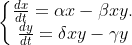
with initial values for x = 10 and y = 10.

The parameter values for alpha, beta, delta and gamma are 1.1, 0.4, 0.1 and 0.4 respectively (mimicking this example).

Attempt to solve problem:

library(sde)
d <- expression((1.1 * x[0] - 0.4 * x[0] * x[1]), (0.1 * x[0] * x[1] - 0.4 * x[1]))
s <- expression(0, 0)
X <- sde.sim(X0=c(10,10), T = 10, drift=d, sigma=s) 
plot(X)

However, this does not seem to generate a nice cyclic behavior of the predator and prey population.

Expected Output

I used the deSolve package in R to generate the expected output.

library(deSolve)
alpha <-1.1
beta <- 0.4
gamma <- 0.1
delta <- 0.4

yini <- c(X = 10, Y = 10) 
Lot_Vol <- function (t, y, parms) {
  with(as.list(y), {
    dX <- alpha * X - beta * X * Y 
    dY <- 0.1 * X * Y - 0.4 * Y
    list(c(dX, dY))
  }) }
times <- seq(from = 0, to = 100, by = 0.01)
out   <- ode(y = yini, times = times, func = Lot_Vol, parms = NULL)
plot(y=out[, "X"], x = out[, "time"], type = 'l', col = "blue", xlab = "Time", ylab = "Animals (#)")
lines(y=out[, "Y"], x = out[, "time"], type = 'l', col = "red")

Question

I think something might be wrong the the drift function, however, I am not sure what. What is going wrong in the attempt to solve this system of ODEs in sde.sim()?

Answer 1

Assuming that not specifying a method takes the first in the list, and that all other non-specified parameters take default values, you are performing the Euler method with step size h=0.1.

As is known on a function that has convex concentric trajectories, the Euler method will produce an outward spiral. As a first order method, the error should grow to size about T*h=10*0.1=1. Or if one wants to take the more pessimistic estimate, the error has size (exp(LT)-1)*h/L, with L=3 in some adapted norm this gives a scale of 3.5e11.

---

Exploring the actual error e(t)=c(t)*h of the Euler method, one gets the following plots. Left are the errors of the components and right the trajectories for various step sizes in the Euler method. The error coefficient the function c(t) in the left plots is scaled down by the factor (exp(L*t)-1)/L to get comparable values over large time intervals, the value L=0.06 gave best balance.

One can see that the actual error

abs(e(t))<30*h*(exp(L*t)-1)/L

is in-between the linear and exponential error models, but closer to the linear one.

---

To reduce the error, you have to decrease the step size. In the call of SDE.sim, this is achieved by setting the parameter N=5000 or larger to get a step size h=10/5000=0.002 so that you can hope to be correct in the first two digits with an error bound of 30*h*T=0.6. In the SDE case you accumulate Gaussian noise of size sqrt(h) in every step, so that the truncation error of O(h^2) is a rather small perturbation of the random number.

Answer 2

By solving Lotka-Volterra system of ODEs (initial value problem) with Runge-Kutta order 4 (RK4) method with the following code, we can achieve faster convergence and more accurate result with small time-step (delat_t=0.01) and obtain the desired plot:

Runge_Kutta_4_update <- function(xn, delta_t, f) {
  xn <- as.numeric(xn)
  k1 <- f(xn) * delta_t
  k2 <- f(xn + k1/2) * delta_t
  k3 <- f(xn + k2/2) * delta_t
  k4 <- f(xn + k3) * delta_t
  return (xn + 1/6 * (k1 + 2*k2 + 2*k3 + k4))
}

f <- function(v) {
  x <- v[1]
  y <- v[2]
  return (c(alpha * x - beta * x * y, delta * x * y - gamma * y))
}

solve_Lotka_Volterra <- function(v0, delta_t=0.01, niter=10000) {
  ts <- c(0)
  vs <- data.frame(prey=v0[1], predtor=v0[2])
  for (i in seq(2, niter)) {
    ts <- c(ts, ts[i-1] + delta_t)
    v <- Runge_Kutta_4_update(vs[i-1, ], delta_t, f)
    vs <- rbind(vs, data.frame(prey=v[1], predtor=v[2]))
  }
  vs['t'] <- ts
  return (vs)
}

alpha <- 1.1 
beta <- 0.4 
delta <- 0.1
gamma <- 0.4
solution_df <- solve_Lotka_Volterra(c(10,10))
library(tidyverse)
solution_df %>% gather('var', 'val', -t) %>% ggplot(aes(t, val, col=var)) + 
  geom_line(lwd=1) + theme_bw() + ggtitle('Solution with Runge-Kutta order-4')