-1

I would like to "walk" through a Excel column and if the the preceding or following cell has the same value or single, mark it with a color. For example:

example pic

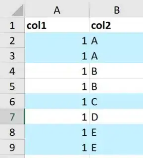
i have get this by creating an auxiliary column.Can anyone goal this without VBA nor an auxiliary column. my solution

OdTu
  • 149
  • 3
  • What do you mean "or single"? Is your goal to alternate cell shading on each group in `col2`? – ashleedawg May 30 '18 at 02:53
  • single --> like row 6. – OdTu May 30 '18 at 02:56
  • Possible duplicate of [Alternating coloring groups of rows in Excel](https://stackoverflow.com/questions/27020/alternating-coloring-groups-of-rows-in-excel) There are various other examples of hoe to do this as well, such as **[this search](https://www.google.com/search?q=excel+alternate+shading+group).** – ashleedawg May 30 '18 at 02:57
  • yes,i want to alternate cell shading on each group in col2. – OdTu May 30 '18 at 02:57
  • thx ,but i want to konw if anyone can goal this without using VBA nor an auxiliary column – OdTu May 30 '18 at 03:05
  • 1
    Look here: https://stackoverflow.com/questions/16492425/excel-conditional-formatting-for-clusters-of-values/16493622#16493622 – teylyn May 30 '18 at 03:15
  • Alright, that's also possible with the help of conditional formatting. See the link from @teylyn or also this one: ["Dynamic Row Shading with Conditional Formatting Formulas"](https://stackoverflow.com/questions/39733229/dynamic-row-shading-with-conditional-formatting-formulas-excel) and others. – ashleedawg May 30 '18 at 03:25
  • thx all.This is confirmed that can't alternate cell shading on each group in col2 without VBA nor an auxiliary column – OdTu May 31 '18 at 08:13

1 Answers1

0

Select ColumnsA:B, clear any CF from it and then HOME > Styles - Conditional Formatting, New Rule..., Use a formula to determine which cells to format and Format values where this formula is true::

=ISODD(SUMPRODUCT(1/COUNTIF($B1:$B$9,$B1:$B$9)))

Format..., select blue Fill, OK, OK.

pnuts
  • 58,317
  • 11
  • 87
  • 139