I have the following ordinary least squares model (OLS) interactive model that I want to extract discrete marginal effects (i.e. the average marginal effect of weight across discrete categories of speed and foreign-build autos) for the triple interactionweight* speed*foreign:
mpg ~ cost + foreign + weight + speed + foreign + cost*foreign + weight*speed + weight*speed*foreign
As one can see, there are three interactions in the model. The variables are specified as follows:
cost is a continuous variable centered at the mean value of all cars on the market, with negative values indicating degrees below the mean and positive values indicating more expensive cars.
foreign is a binary variable, 1 foreign/0 domestic
weight is a continuous variable
speed is a factor variable indicating how fast the car goes in three categories, low-medium-high. Low is the base-line category (omitted category).
The quantity of interest is the triple interaction in the model: weight*speed*foreign. I use the following code to estimate the model and extract the relevant coefficients and variance covariance matrix. I want to use the following procedure from Berry et al. (2016) article: "Improving Tests of Theories Positing Interaction", using the following chart:Marginal Effects Formulation
I extract the relevant coefficients needed to derive the marginal effects and the variance-covariance matrix using the following code:
m <- lm(mpg ~ cost + foreign + weight + speed + foreign + cost*foreign + weight*speed + weight*speed*foreign, data=x)
beta.hat <- coef(m)
cov <-  vcov(m)
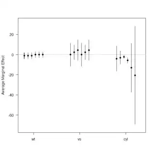
Ultimately, I want a data frame containing the average marginal effect of weight across the different discrete categories of speed & foreign, with the end goal being a dot-plot showing discrete marginal effects. Following the image, I know how to derive the marginal effects for the two non-omitted categories of the factor variable (speed). For example, I think this is done correctly for the "high" speed":
z0 <- seq(0,1,1) #This captures the two-categories of the Z conditioning variable of foreign
dy.dx <-  beta.hat["weight"] + beta.hat["weight*speed=High"] + beta.hat["weight*foreign*speed=High"]*z0 # Discrete Marginal Effect
se.dy.dx <- sqrt(cov["weight", "weight"] + z0^2*cov["weight * speed=High", "weight * speed=High"] + z0^2*cov["foreign * weight", "foreign * weight"] + z0^2*z0^2*cov["foreign * weight * speed=High", "foreign * weight * speed=High"] + 2*z0*cov["weight","weight * speed=High"] + 2*z0*cov["weight","foreign * weight"] + 2*z0*z0*cov["weight","foreign * weight * speed=High"] + 2*z0*z0*cov["weight * speed=High","foreign * weight"] + 2*z0*z0^2*cov["weight * speed=High","foreign * weight * speed=High"] + 2*z0*z0^2*cov["foreign * weight","foreign * weight * speed=High"]) #Compute Standard Errors for MEs of foreign and domestic cars
The main question I have is how do I derive the average marginal effects of weight for the omitted category of speed? I understand that this is captured by the weight*speed constituent term, but do I need to consider the triple interaction in calculating the standard errors, dy.dx of the estimates? Is this an adequate solution given Berry et al.'s table in row 3?
