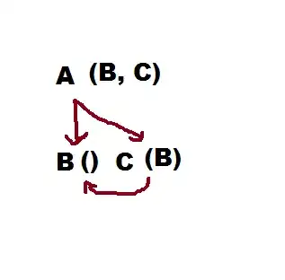
My solution with some explanation below.
library(gapminder)
library(purrr)
library(tidyr)
library(broom)

nest_data <- gapminder %>% group_by(continent) %>% nest(.key = by_continent)
First question was: how to nest by_country inside the nested by_continent
Great solution by @aosmith on the comments
nested_again<-
nest_data %>% mutate(by_continent = map(by_continent, ~.x %>%
                                          group_by(country) %>%
                                          nest(.key = by_country)))
# Level 1
nested_again
# # A tibble: 5 × 2
# continent      by_continent
# <fctr>            <list>
#   1      Asia <tibble [33 × 2]>
#   2    Europe <tibble [30 × 2]>
#   3    Africa <tibble [52 × 2]>
#   4  Americas <tibble [25 × 2]>
#   5   Oceania  <tibble [2 × 2]>

# Level 2
nested_again %>% unnest %>% slice(1:2)
# # A tibble: 2 × 3
# continent     country        by_country
# <fctr>      <fctr>            <list>
#   1      Asia Afghanistan <tibble [12 × 4]>
#   2      Asia     Bahrain <tibble [12 × 4]>
Second question: how to apply a regression model at a deeper level (and save the models on the tibble, I suppose)
Solution by @aosmith (which I'm calling sol1)
sol1<-mutate(nested_again, models = map(by_continent, "by_country") %>%
         at_depth(2, ~lm(lifeExp ~ year, data = .x)))

sol1
# # A tibble: 5 × 3
# continent      by_continent      models
# <fctr>            <list>      <list>
#   1      Asia <tibble [33 × 2]> <list [33]>
#   2    Europe <tibble [30 × 2]> <list [30]>
#   3    Africa <tibble [52 × 2]> <list [52]>
#   4  Americas <tibble [25 × 2]> <list [25]>
#   5   Oceania  <tibble [2 × 2]>  <list [2]>

sol1 %>% unnest(models)
# Error: Each column must either be a list of vectors or a list of data frames [models]
sol1 %>% unnest(by_continent) %>% slice(1:2)
# # A tibble: 2 × 3
#   continent     country        by_country
#      <fctr>      <fctr>            <list>
# 1      Asia Afghanistan <tibble [12 × 4]>
# 2      Asia     Bahrain <tibble [12 × 4]>
The solution is doing what it is supposed to, but there's no easy way to filter by country, because that information is nested in the level 2.
I propose the solution 2, based on @aosmith's solution to the first question:
sol2<-nested_again %>% mutate(by_continent = map(by_continent, ~.x %>%
                  mutate(models = map(by_country, ~lm(lifeExp ~ year, data = .x) )) ))
sol2
# # A tibble: 5 × 2
#   continent      by_continent
#      <fctr>            <list>
# 1      Asia <tibble [33 × 4]>
# 2    Europe <tibble [30 × 4]>
# 3    Africa <tibble [52 × 4]>
# 4  Americas <tibble [25 × 4]>
# 5   Oceania  <tibble [2 × 4]>

sol2 %>% unnest %>% slice(1:2)
# # A tibble: 2 × 4
#   continent     country        by_country   models
#      <fctr>      <fctr>            <list>   <list>
# 1      Asia Afghanistan <tibble [12 × 4]> <S3: lm>
# 2      Asia     Bahrain <tibble [12 × 4]> <S3: lm>

sol2 %>% unnest %>% unnest(by_country) %>% colnames
# [1] "continent" "country"   "year"      "lifeExp"   "pop"
# [6] "gdpPercap"

# get model by specific country
sol2 %>% unnest %>% filter(country == "Brazil") %$% models %>% extract2(1)
# Call:
#   lm(formula = lifeExp ~ year, data = .x)
#
# Coefficients:
#   (Intercept)         year
# -709.9427       0.3901

# summary with broom::tidy
sol2 %>% unnest %>% filter(country == "Brazil") %$% models %>%
  extract2(1) %>% tidy
#          term     estimate    std.error statistic      p.value
# 1 (Intercept) -709.9426860 10.801042821 -65.72909 1.617791e-14
# 2        year    0.3900895  0.005456243  71.49417 6.990433e-15
We can tidy all the models and save in the data to use for plotting or filter
sol2 %<>% mutate(by_continent = map(by_continent, ~.x %>%
        mutate(tidymodels = map(models, tidy )) ))

sol2 %>% unnest %>% unnest(tidymodels) %>%
  ggplot(aes(country,p.value,colour=continent))+geom_point()+
  facet_wrap(~continent)+
  theme(axis.text.x = element_blank())

selc <- sol2 %>% unnest %>% unnest(tidymodels) %>% filter(p.value > 0.05) %>%
  select(country) %>% unique %>% extract2(1)

gapminder %>% filter(country %in% selc ) %>%
  ggplot(aes(year,lifeExp,colour=continent))+geom_line(aes(group=country))+
  facet_wrap(~continent)

aaaaand, we can use the models
m1 <- sol2 %>% unnest %>% slice(1) %$% models %>% extract2(1)

x <- sol2 %>% unnest %>% slice(1) %>% unnest(by_country) %>% select(year)

pred1 <- data.frame(year = x, lifeExp = predict.lm(m1,x))

sol2 %>% unnest %>% slice(1) %>% unnest(by_country) %>%
  ggplot(aes(year, lifeExp )) + geom_point() +
  geom_line(data=pred1)

In this case there's really no good reason to use this double nesting (besides learning how to to it, of course), but I found a case in my work where it is extremely valuable, specifically when you need a function to work on a 3rd level, grouped by levels 1 and 2, and save in level 2 - of course for this we could also use a for loop on level 1, but what's the fun in that ;) I'm not really sure how this "nested" map performs compared to for loop + map, but I'll test it next.
Benchmark
It looks like they do not differ much
# comparison map_map with for_map
map_map<-function(nested_again){
nested_again %>% mutate(by_continent = map(by_continent, ~.x %>%
  mutate(models = map(by_country, ~lm(lifeExp ~ year, data = .x) )) )) }

for_map<-function(nested_again){ for(i in 1:length(nested_again[[1]])){
  nested_again$by_continent[[i]] %<>%
  mutate(models = map(by_country, ~lm(lifeExp ~ year, data = .x) )) }}

res<-microbenchmark::microbenchmark(
  mm<-map_map(nested_again), fm<-for_map(nested_again) )

res
# Unit: milliseconds
#                         expr      min       lq     mean   median       uq      max neval cld
#  mm <- map_map(nested_again) 121.0033 144.5530 160.6785 155.2389 174.2915 240.2012   100   a
#  fm <- for_map(nested_again) 131.4312 148.3329 164.7097 157.6589 173.6480 455.7862   100   a

autoplot(res)


