Fitting parameters do not converge, but nlsLM() stops

Question

In R, I'm trying to fit a series of data to a curve given by the theory, which is:

y(x) = (1 + fitbeta * x)^(-fitgamma)

In theory this should work and others have used this formula successfully. However, I cannot seem to make my fit parameters converge, no matter the starting conditions or options I try.

Below is a reproducible example. Note that I am using the package minpack.lm, which is a nice improvement over nls() which - by the way - throws a Missing value or an infinity produced when evaluating the model error at me when I try to use it (with the same settings).

This may be a trivial question for most of you, but I do not know nls() at all and I'm just starting to use it. There must be something super-simple I'm missing!

Here's the code:

#Libraries:
library(ggplot2)    #Plots
library(minpack.lm) #Non linear formula fits

#Reproducible example parameters:
startbeta=0.001
startgamma=-10
X <- c(1, seq(2,240,2)) #Vector of durations in hours
Y <- c(1, 0.999349067282531, 0.997149973857984, 0.993613390445064,
0.988771983639396, 0.982724692889081, 0.975628661286657, 0.96751072812657,
0.958414894569813, 0.948463753530251, 0.93767394420049, 0.926259971613655,
0.91433495083748, 0.901955098152661, 0.889290679032582, 0.876927340669535,
0.864697870521103, 0.852357436802833, 0.839855401239168, 0.827134255036668,
0.814227652658426, 0.801278249082419, 0.788355912487271, 0.775514097293561,
0.762891867628759, 0.750380786683852, 0.738018762182673, 0.725799137700828,
0.713720035497274, 0.701808749767634, 0.690046213599144, 0.678484705844808,
0.667111445204795, 0.655977696751697, 0.645116379924585, 0.634460211234775,
0.623985607991471, 0.613706080277076, 0.603604313599018, 0.593685433942668,
0.58395373490791, 0.574696581531438, 0.565639259757887, 0.556883924877305,
0.54829105550864, 0.539882579975057, 0.531669333311634, 0.523789998486779,
0.516140798533169, 0.508732414242052, 0.501549858546355, 0.494581375404643,
0.487806083201077, 0.481215549260729, 0.475344757534521, 0.469883620527239,
0.464505182123833, 0.459295389779093, 0.454254664927743, 0.449272635346615,
0.444353923395879, 0.439502685117945, 0.434723592424652, 0.430300205554656,
0.425950322720235, 0.421651255977861, 0.417403585324494, 0.413205553596921,
0.409056611802817, 0.404966487426596, 0.400979187396173, 0.39721419353495,
0.393559414540655, 0.389971147514211, 0.386435641037176, 0.382947750185137,
0.379497143530884, 0.376143019983175, 0.373016368099911, 0.369904788649644,
0.366813427145508, 0.363784767175811, 0.360999911892512, 0.358249758228913,
0.355539445964091, 0.352899943455576, 0.35037387237155, 0.347925865476795,
0.345529621963385, 0.343187675737988, 0.340930763575173, 0.338722557572396,
0.336557943062853, 0.334418098646777, 0.332805911075547, 0.33117666406428,
0.329516391536038, 0.327847961775104, 0.32615922691243, 0.324473380427564,
0.322807248963926, 0.321128906622371, 0.319431589984492, 0.317714245126025,
0.315983206323488, 0.314233066510948, 0.312462213805877, 0.310672914913813,
0.308902798280917, 0.307149178519641, 0.305387995487162, 0.303621881791372,
0.301859643176666, 0.300098168944162, 0.298340765140062, 0.296633192262476,
0.294981140721158, 0.293349312493173, 0.291718961012827, 0.290087159821697,
0.288466970001273)

#Plot function:
ggp <- function(b=fitbeta, g=fitgamma) {
  gg <- ggplot(data.frame(x = c(0, 240)), aes(x)) +
    stat_function(fun = function(x) (1 + b * x)^(-g), geom = "line") +
    geom_line(data=data.frame(x=X, y=Y), aes(y=y, x=x), colour="red")
  print(gg)
}

#Fit:
nlc <- nls.control(maxiter = 1000)
fit <- nlsLM(y ~ I((1 + fitbeta * x)^(-fitgamma)), #Function from NERC(1975)
            data = data.frame(y=Y, x=X),
            start = list(fitbeta = startbeta, fitgamma=startgamma),
            trace=TRUE, control=nlc)
  #Get the coefficients of the fit
  fitbeta  <- coef(fit)[1]
  fitgamma <- coef(fit)[2]

#Plot:
ggp()

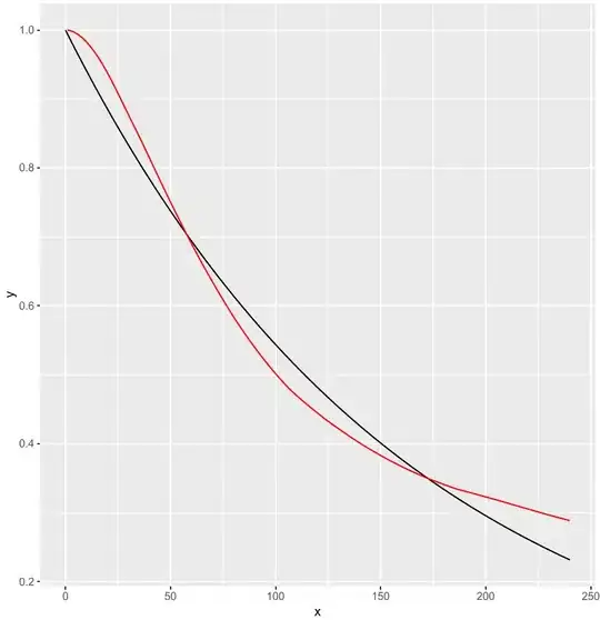
The result is not too shabby: (in black the fitted curve, in red the input data)

However, if I look at the nlsLM() trace:

...
It.   64, RSS =    0.13003, Par. = -1.37045e-05   -444.272
It.   65, RSS =   0.130024, Par. = -1.33717e-05   -455.143
It.   66, RSS =   0.130014, Par. = -1.30753e-05   -465.508
It.   67, RSS =   0.130006, Par. = -1.29238e-05   -471.145
It.   68, RSS =       0.13, Par. = -1.26237e-05   -482.163
It.   69, RSS =   0.129991, Par. = -1.23554e-05   -492.681
It.   70, RSS =   0.129984, Par. = -1.22119e-05   -498.639
It.   71, RSS =   0.129979, Par. = -1.19291e-05   -510.269
It.   72, RSS =    0.12997, Par. = -1.16755e-05   -521.396
It.   73, RSS =   0.129964, Par. = -1.15447e-05   -527.488
It.   74, RSS =   0.129959, Par. = -1.12865e-05   -539.368
It.   75, RSS =   0.129951, Par. = -1.10541e-05   -550.747
It.   76, RSS =   0.129945, Par. = -1.09312e-05   -557.117
It.   77, RSS =   0.129941, Par. = -1.06886e-05   -569.567
It.   78, RSS =   0.129933, Par. = -1.04713e-05   -581.433
It.   79, RSS =   0.129928, Par. = -1.03588e-05   -587.931
It.   80, RSS =   0.129924, Par. = -1.01368e-05   -600.613
It.   81, RSS =   0.129917, Par. = -9.93656e-06   -612.764
It.   82, RSS =   0.129912, Par. = -9.82966e-06   -619.607
It.   83, RSS =   0.129908, Par. = -9.61868e-06   -632.993
It.   84, RSS =   0.129902, Par. = -9.42521e-06   -646.024
It.   85, RSS =   0.129896, Par. = -9.24949e-06   -658.345
It.   86, RSS =   0.129891, Par. = -9.14794e-06   -665.812
It.   87, RSS =   0.129888, Par. = -8.9485e-06   -680.423
It.   88, RSS =   0.129882, Par. = -8.7693e-06    -694.38
It.   89, RSS =   0.129876, Par. = -8.58442e-06   -709.315
It.   90, RSS =   0.129871, Par. = -8.41437e-06   -723.697
It.   91, RSS =   0.129866, Par. = -8.25997e-06   -737.276
It.   92, RSS =   0.129862, Par. = -8.17745e-06     -744.9
It.   93, RSS =   0.129859, Par. = -8.01476e-06   -759.809

It does not actually look like it is converging, the two parameters continue to change and actually diverge. What is happening here and why does the fitter stop, if the parameters are not stable?

Answer 1

This is not a solution, but some food for thoughts:

In my experience, if you have serious errors from nls, using nlsLM is not a good fix as it will give you usually a result, but often not a good result. An alternative approach would be using a whole bunch of optimizers and check if they can somewhat agree on a solution.

library(optimx)
fun <- function(x, b, c) (1 + b * x)^(-log(c))
fun1 <- function(pars) sum((Y - fun(X, pars["b"], pars["c"]))^2)
fits <- optimx(c(b = 0.001, c = log(10)), fun1, control = list(all.methods = TRUE))
fits
#                      b         c         value fevals gevals niter convcode  kkt1  kkt2 xtimes
#BFGS        0.009277751  2.745042  2.453159e-01     88     20    NA        0 FALSE  TRUE   0.02
#CG          0.012242506  2.300605  3.184743e-01    171     19    NA        0 FALSE  TRUE   0.00
#Nelder-Mead 0.004664550  5.396015  1.427017e-01    175     NA    NA        0 FALSE FALSE   0.00
#L-BFGS-B             NA        NA 8.988466e+307     NA     NA    NA     9999    NA    NA   0.00
#nlm         0.001000000  2.302585 1.797693e+308     NA     NA     0        0    NA    NA   0.00
#nlminb      0.001674994 58.216382  1.081060e-01    123    191    89        0  TRUE FALSE   0.00
#spg         0.019577915  2.286535  1.448918e+00      7     NA     4        3 FALSE FALSE   0.14
#ucminf      0.001000000  2.302585  2.153628e+01      1      1    NA        0 FALSE FALSE   0.00
#Rcgmin               NA        NA 8.988466e+307     NA     NA    NA     9999    NA    NA   0.00
#Rvmmin               NA        NA 8.988466e+307     NA     NA    NA     9999    NA    NA   0.00
#newuoa               NA        NA 8.988466e+307     NA     NA    NA     9999    NA    NA   0.00
#bobyqa      0.024625964  2.801075  5.831466e+00     23     NA    NA        0    NA    NA   0.00
#nmkb                 NA        NA 8.988466e+307     NA     NA    NA     9999    NA    NA   0.00
#hjkb        0.001000000  2.302585  2.153628e+01      1     NA     0     9999    NA    NA   0.00

plot(X, Y)
curve(fun(x, fits["BFGS", "b"], fits["BFGS", "c"]), add = TRUE)
curve(fun(x, fits["CG", "b"], fits["CG", "c"]), add = TRUE, col = "blue")
curve(fun(x, fits["Nelder-Mead", "b"], fits["Nelder-Mead", "c"]), add = TRUE, col = "red")
curve(fun(x, fits["nlminb", "b"], fits["nlminb", "c"]), add = TRUE, col = "green")

As you see, most of the converging optimizers give quite different parameter estimates and non of these fits can be considered good. I suspect that this is not merely a result of bad starting values, but that your data just doesn't conform to the model. In particular, it doesn't look like the model can represent the slightly sigmoidal shape of your data.