A first suggestion that somewhat sidesteps the solution I'm looking for is to combine all my data into one data table and use facet_grid on my variable and simulation
ggplot() + ... + facet_grid(variable~simulation, scales = 'free_y')
This produces a fine looking plot that displays the data in one figure, but can become unwieldy when considering many simulations.
To 'hack' the plotting into producing what I want, I first determined which limits I desired for each weather variable. These limits were found by looking at the greatest extents for all simulations of interest. Once determined I created a small data table with the same columns as my simulation data and appended it to the end. My simulation data had the structure
    'year' 'month' 'variable' 'run' 'mean'
     1973     1     'rhmax'     1    65.44
     1973     2     'rhmax'     1    67.44
     ...     ...      ...      ...    ...
     2011    12    'windmin'   200    0.4
So I created a new data table with the same columns
    ylims.sims <- data.table(year = 1, month = 13,
    variable =  rep(c('rhmax','rhmin','sradmean','tmax','tmin','windmax','windmin'), each = 2),
    run = 201, mean = c(20, 100, 0, 80, 100, 350, 25, 40, 12, 32, 0, 8, 0, 2))
Which gives
    'year' 'month' 'variable' 'run' 'mean'
       1     13     'rhmax'    201    20
       1     13     'rhmax'    201    100
       1     13     'rhmin'    201    0
       1     13     'rhmin'    201    80
       1     13    'sradmean'  201    100
       1     13    'sradmean'  201    350
       1     13     'tmax'     201    25
       1     13     'tmax'     201    40
       1     13     'tmin'     201    12
       1     13     'tmin'     201    32
       1     13    'windmax'   201    0
       1     13    'windmax'   201    8
       1     13    'windmin'   201    0
       1     13    'windmin'   201    2
While the choice of year and run is aribtrary, the choice of month need to be anything outside 1:12. I then appended this to my simulation data
    sim1data.ylims <- rbind(sim1data, ylims)
    ggplot() + geom_boxplot(data = sim1data.ylims, aes(x = factor(month), y = mean)) +
    facet_wrap(~variable, scale = 'free_y') + xlab('month') +
    xlim('1','2','3','4','5','6','7','8','9','10','11','12')
When I plot these data with the y limits, I limit the x-axis values to those in the original data. The appended data table with y limits has month values of 13. As ggplot still scales axes to the entire dataset, even when the axes are limited, this gives me the y limits I desire. Important to note that if there are data values greater than the limits you specify, this will not work.
Before: Notice the differences in the y limits for each weather variable between the panels.
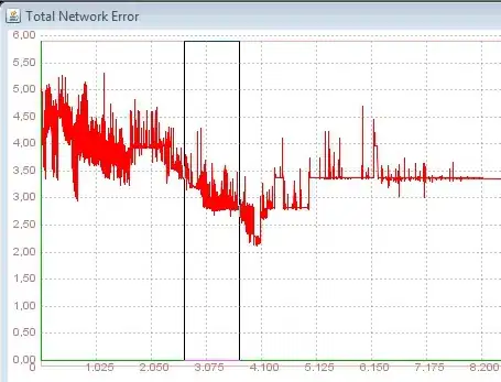
After: Now the y limits remain consistent for each weather variable between the panels.


I hope to edit this post in the coming days and add a reproducible example for better explanation. Please comment if you've heard anything about adding this functionality to ggplot.
 When I compare between different plot panels, its nice to have consistent axes. Unfortunately ggplot provides no way of setting the individual limits of each plot within a panel plots. It defaults to using the range of given data. The Google Group discussion linked above discusses this shortcoming, but I was unable to find any updates as to whether this could be added. Is there a way to trick ggplot to set the individual limits?