Grouping price ranges

Question

I am trying to group some price ranges from an .ods file, but have no idea how to do that.

e.g. I have a column with different prices like this:

What I want is to tell Calc to group everything from 0,00~10,99 and output text 0-10 and everything from 11,00~20,00 and output text 11-20, so the final output would be:

col1    col2
11,61   11-20
6,15    0-10
13,68   11-20
7,69    0-10
6,00    0-10

An arithmetic solution is quite difficult, since the intervals are different (0 to 10,99 is a bigger interval than 11,00 to 20,99). So i ask you to narrow down the problem: must a solution cover values greater than 20, or is it enough to differentiate between values smaller or greater than 11,00? — tohuwawohu, Apr 13 '14 at 17:25
values can get up to 100. The ideal solution is a grouping like0-9 9-19 19-29 29-39 39-59 59-79 79-100 — user3292026, Apr 13 '14 at 17:58
I've modified my solution so it should work for 0-9, 9-19. 19-29, 29-39, 39-49 and so on. Handling the output differently for values > 39 would be possible, but this would make the formula even more complex. — tohuwawohu, Apr 15 '14 at 15:40

tohuwawohu · Answer 1 · 2014-04-19T10:01:29.680

You can use the functions ROUNDDOWN() and ROUNDUP() with a negative count to get the next multiple of 10 (-1), 100 (-2) or 1000 (-3). It reduces the accuracy of a certain value by squares of 10. So, rounding to the previous or next multiple of 10 is done using:

=ROUNDDOWN(<yourvalue>; -1)

and

=ROUNDUP(<yourvalue>; -1)

respectively (take care to adapt the formula argument separators to commata (,) if this is required by the i18y your're using).

So, =ROUNDDOWN(11,61; -1) will result in 10, and =ROUNDUP(11,61; -1) will give you 20. This way, you can "calculate" the appropriate group for each value (example for value in A1):

=CONCATENATE(ROUNDDOWN($A1; -1)+1;"-";ROUNDUP($A1;-1))

To split it up on multiple lines:

=CONCATENATE(              # Result will be a concatenated string
    ROUNDDOWN($A1;-1)+1;   # first value: previous multiple of 10, +1;
    "-";                   # second value: literal "-"
    ROUNDUP($A1;-1)        # third value: next multiple of 10
)

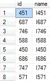
With your example data, this results in:

enter image description here

EDIT:

For a grouping 0-9, 9-19 and so on, the following formula should work:

=CONCATENATE(ABS(ROUNDDOWN($A2+1; -1)-1);"-";ROUNDUP($A2+1,01;-1)-1)

enter image description here

EDIT2:

For a solution using the IF() function, you could use:

=IF(A2 < 9;"0-9";IF(A2 < 19; "9-19";IF(A2 < 29; "19-29";"more than 29")))

For grouping of values greater than 29, you will have to add according IF clauses replacing the string "more than 29" by additional checks. Every grouping range will require its own IF clause.

Hi and thanks for the quick answer. One problem I found though it that eg. 10,01 should belong to 1-10 and not 11-20 — user3292026, Apr 13 '14 at 16:10
Oh, yes, you're completely right - i will try to adapt the formula to that need. — tohuwawohu, Apr 13 '14 at 17:11
Hi, sorry for the late reply(was away). Although this seems to work OK, would it not be easer if calc used < and > to find a range and then output the 29-39 text — user3292026, Apr 18 '14 at 21:20
Using IF would be possible, too. The advantage of a formula using the current values is that it works for every initial value. With IF, you would have to adapt the formula if the initial values grow bigger than 100, for example. My solution works for every initial positive value. — tohuwawohu, Apr 19 '14 at 07:06

Grouping price ranges

1 Answers1