Overlay histograms in R

Question

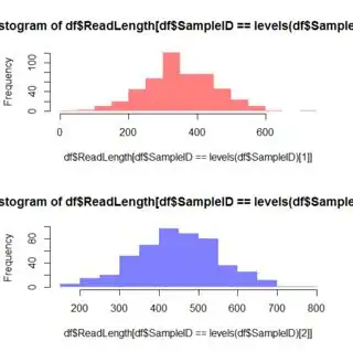
I want to plot a histogram of lengths based on locations. I am trying to overlay the histogram where data of one location is one color and the other location is a different color.

Here is the R code I have so far that just plots the histogram:

    fasta<-read.csv('fastadata.csv',header = T)
    norton<-fasta[fasta$SampleID == ">P.SC1Norton-28F",]
    cod<-fasta[fasta$SampleID == ">P.SC4CapeCod-28F ",]
    bins <- seq(200, 700, by=25)
    hist(fasta[,3], breaks=bins, main="Histogram of ReadLengths of a set bin size for Cape Cod and Norton", xlab="ReadLengths")

I keep seeing ggplot used, but I am unsure how to use this function within one table and using the binning I used.

Output of dput(head(fasta)):

structure(list(SampleID = structure(c(2L, 2L, 2L, 2L, 2L, 2L), .Label = c(">P.SC1Norton-28F",">P.SC4CapeCod-28F"), class = "factor"), SeqName = structure(c(5674L, 5895L, 5731L, 5510L, 4461L, 5648L), .Label = c("IJO4WN203F00DQ", "IKTXKCP03HKQ5E"), class = "factor"), ReadLength = c(394L, 429L, 437L, 438L, 459L, 413L)), .Names = c("SampleID", "SeqName", "ReadLength"), row.names = c(NA, 6L), class = "data.frame")

I should have probably asked for at least two different IDs I guess. — Rich Scriven, Mar 06 '14 at 07:25

score 10 · Accepted Answer · answered Mar 06 '14 at 07:31

10

Since you mentioned ggplot, you have several options.

# make up some data
set.seed(1)
sampleID <- c(">P.SC1Norton-28F",">P.SC4CapeCod-28F")
df <- data.frame(SampleID=rep(sampleID,each=500),
                 ReadLength=round(c(rnorm(500,350,100),rnorm(500,450,100))))

library(ggplot2)
ggplot(df) +
  geom_histogram(aes(x=ReadLength, fill=SampleID), 
                 colour="grey50", alpha=0.5, position="identity")

ggplot(df) +
  geom_histogram(aes(x=ReadLength, fill=SampleID), position="dodge")

ggplot(df) +
  geom_histogram(aes(x=ReadLength, fill=SampleID))+
  facet_wrap(~SampleID,nrow=2)

answered Mar 06 '14 at 07:31

jlhoward

58,004
7
97
140

Thank You this really help.For the ggplot is this a library package that I would have to install additionally? – user3018479 Mar 06 '14 at 07:34
Right. `install.packages("ggplot2")`. – jlhoward Mar 06 '14 at 07:36

Thomas · Answer 2 · 2014-03-06T09:31:10.217

Use the add=TRUE parameter in a second call to hist. Also, using an alpha-transparent color will probably help.

hist(norton[,3], breaks=bins, main="Histogram of ReadLengths of a set bin size for Cape Cod and Norton", 
     xlab="ReadLengths", col=rgb(1,0,0,.5), border=NA)
hist(cod[,3], breaks=bins, col=rgb(0,0,1,.5), add=TRUE, border=NA)

Here's an update using @jlhoward's data. Note that the axis labels and headings are messy by default:

layout(1:2)
hist(df$ReadLength[df$SampleID==levels(df$SampleID)[1]],
     col=rgb(1,0,0,.5), border=NA)
hist(df$ReadLength[df$SampleID==levels(df$SampleID)[2]],
     col=rgb(0,0,1,.5), border=NA, add=TRUE)

enter image description here

hist(df$ReadLength[df$SampleID==levels(df$SampleID)[1]],
     col=rgb(1,0,0,.5), border=NA)
hist(df$ReadLength[df$SampleID==levels(df$SampleID)[2]],
     col=rgb(0,0,1,.5), border=NA)

enter image description here

Thank You! I get color, but I am trying to have 2 colors. One color for each locations. Do I just change the col in the second hist color? — user3018479, Mar 06 '14 at 07:19

score 0 · Answer 3 · answered Aug 14 '22 at 16:15

Another really simple way of plotting overlay histograms is using the ggpubr package with gghistogram function like this:

library(ggpubr)
set.seed(1)
sampleID <- c(">P.SC1Norton-28F",">P.SC4CapeCod-28F")
df <- data.frame(SampleID=rep(sampleID,each=500),
                 ReadLength=round(c(rnorm(500,350,100),rnorm(500,450,100))))
gghistogram(df, x = "ReadLength",
            fill = "SampleID",
            palette = c("red", "blue"))
#> Warning: Using `bins = 30` by default. Pick better value with the argument
#> `bins`.

^{Created on 2022-08-14 by the reprex package (v2.0.1)}

This could easily be extended to for example 3 histograms:

library(ggpubr)
set.seed(1)
sampleID <- c(">P.SC1Norton-28F",">P.SC4CapeCod-28F", ">P.SC6CapeCod-28F")
df <- data.frame(SampleID=rep(sampleID,each=500),
                 ReadLength=round(c(rnorm(500,350,100),rnorm(500,450,100),rnorm(500,550,100))))
gghistogram(df, x = "ReadLength",
            fill = "SampleID",
            palette = c("red", "blue", "green"))
#> Warning: Using `bins = 30` by default. Pick better value with the argument
#> `bins`.

^{Created on 2022-08-14 by the reprex package (v2.0.1)}

Overlay histograms in R

3 Answers3

Linked