Plotting functions at a specific y-interval

Question

I need to plot a few exponential curves on the same plot - with the constraint that the plot ends at y=1.

For reference, here is the code:

from numpy import arange
from matplotlib import pyplot as plt

T = arange(60,89)
curve1 = 2**(T - 74)
curve2 = 2**(T - 60)
plt.plot(T,curve1 )
plt.plot(T,curve2 )
plt.show()

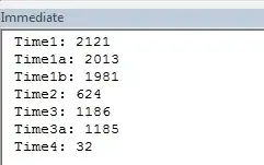
Here's the result: curves 1 and 2 The second curve is just barely visible, since the values are comparatively so low.

The problem I'm having is that all of these curves blow up to 700000+ fairly rapidly, but I'm only interested in the range being (0,1). How do I plot just these bits, but with nice smooth curves (so that one curve doesn't just stop halfway along)?

Are you just asking how to set the y-limits of the plot? Or how to plot only the portions of the curves less than 1? (i.e. `plt.plot(T[data < 1], data[data < 1])` vs `plt.ylim([0, 1])`) — Joe Kington, Jan 20 '14 at 16:03
I just want the portions of the curves less than 1, but without an abrupt stop in any of the curves. — Tom Kealy, Jan 20 '14 at 16:08
Do you want to do this only for these specific curves? Or are you looking for a generic method? — loopbackbee, Jan 20 '14 at 16:13
@goncalopp a generic method would be nice, but I just set plt.ylim([0,1]) for now. — Tom Kealy, Jan 20 '14 at 16:14
In the future, it would be nice if you posted a complete _working_ example of your code. At the moment your code fails for many reasons, `succ`, `succ1` are not defined, `T` is not a numpy array and thus can't be operated on as in `T-74`, etc... It is also not _minimial_, do we really need to see the legend to answer the question? It also helps to spell check the title :) — Hooked, Jan 20 '14 at 16:55
@goncalopp Thank you for editing, the question looks better. A small quibble, it may be dangerous to shadow the python builtin `range` with the numpy version `arange`. For this small example it is fine, but in general it's considered bad practice. — Hooked, Jan 20 '14 at 18:26
@Hooked You're right, I kept it because it seemed to be what the original code was doing. While they're mostly cross-compatible (one returns a list, the other an array), one may rely on `range` returning a list and using list functions. — loopbackbee, Jan 20 '14 at 18:35

score 3 · Answer 1 · answered Jan 20 '14 at 16:13

3

This one was really easy: sorry to have wasted time on it.

Just set the y limits to be [0,1] via

plt.ylim([0,1])

and you're done.

answered Jan 20 '14 at 16:13

Tom Kealy

2,537
2
27
45

1

I don't think you should apologize, there's a non-trivial problem within this question: how to select the proper range (your `T`) such that the curve is smooth and there's no wasted computation. If you wanted a generic method, evaluating the expressions using `sympy` would probably be the way to go – loopbackbee Jan 20 '14 at 16:16
@goncalopp Ideally that's what I'd like - this just cuts the curve off after 1, spoiling the smoothness of the curves I'm expecting. – Tom Kealy Jan 20 '14 at 16:20
You'll get a "smoother" curve by plotting more points - since it jumps so rapidly having only 100 plotting points makes it unlikely to see the transition in any other way but a step function. – Hooked Jan 20 '14 at 16:57
@Hooked 100 points are absolutely enough to plot these functions, *if you make good use of them*. It's unnecessary to plot the regions where the functions are undefined, or where they are out of the bounds of the plot (see my answer) – loopbackbee Jan 20 '14 at 18:02
@goncalopp Yes 100 points is sufficient, _provided you know how to make good use of them_. A priori, you often don't know where the function changes and you can't always rely on an analytical (sympy) solution to solve for it. The suggestion to use more points is motivated by the fact that the time difference between plotting 100 vs 1000 points is (often) negligible. Once you have some idea of the function growth you can certainly optimize it. – Hooked Jan 20 '14 at 18:20

score 3 · Accepted Answer · edited Jul 05 '14 at 12:43

As you've found, this is easy to do if you adjust the range (T) for each function you add. However, if you need to change the functions, you'll need to recheck it.

The problem you're dealing with, generically, is calculating the x-range of some functions given their y-range - or, as a mathematician may put it, determining the domain of a function that corresponds to a range of its image. While, for a arbitrary function, this is impossible, it's possible if your function is injective, as is the case.

Let's say we have a function y=f(x), and the yrange is [y1,y2]. The x-range will be [f^(-1)(y1), f^(-1)(y2] (f^-1 being the inverse function of f)

Since we have multiple functions that we need to plot, the x_range is simply the greatest range - of all - the lower portion of the final range is the minimum of the lower portion of all the ranges, and the upper portion is the maximum of the upper portions.

Here's some code that exemplifies all this, by taking as a parameter the number of steps, and calculating the proper T over the x-range:

from numpy import arange
from matplotlib import pyplot as plt
from sympy import sympify, solve

f1= '2**(T - 74)' #note these are strings
f2= '2**(T - 60)'

y_bounds= (0.001, 1) #exponential functions never take 0 value, so we use 0.001
mm= (min, max)
x_bounds= [m(solve(sympify(f+"-"+str(y)))[0] for f in (f1,f2)) for y,m in zip(y_bounds, mm)]
print x_bounds

N_STEPS=100 #distributed over x_bounds
T = arange(x_bounds[0], x_bounds[1]+0.001, (x_bounds[1]-x_bounds[0])/N_STEPS)

curve1 = eval(f1) #this evaluates the function over the range, by evaluating the string as a python expression
curve2 = eval(f2)
plt.plot(T,curve1)
plt.plot(T,curve2)
plt.ylim([0,1])
plt.show()

The code outputs both the x-range (50.03, 74) and this plot: final plot of two curves

score 3 · Answer 3 · answered Jan 20 '14 at 18:29

In addition to the other answers, it may be worth plotting on a log-scale, since the growth of your functions is essentially exponential. For example:

from numpy import arange
from matplotlib import pyplot as plt

T = arange(60,89)
curve1 = 2**(T - 74)
curve2 = 2**(T - 60)
plt.semilogy(T,curve1 )
plt.semilogy(T,curve2 )
plt.show()

enter image description here

Plotting functions at a specific y-interval

3 Answers3