4

Suppose I have to estimate coefficients a,b in regression:

y=a*x+b*z+c

I know in advance that y is always in range y>=0 and y<=x, but regression model produces sometimes y outside of this range.

Sample data:

mydata<-data.frame(y=c(0,1,3,4,9,11),x=c(1,3,4,7,10,11),z=c(1,1,1,9,6,7))
round(predict(lm(y~x+z,data=mydata)),2) 
    1     2     3     4     5     6 
-0.87  1.79  3.12  4.30  9.34 10.32 

First predicted value is <0.

I tried model without intercept: all predictions are >0, but third prediction of y is >x (4.03>3)

round(predict(lm(y~x+z-1,data=mydata)),2)
   1    2    3    4    5    6 
0.76 2.94 4.03 4.67 8.92 9.68 

I also considered to model proportion y/x instead of y:

mydata$y2x<-mydata$y/mydata$x
round(predict(lm(y2x~x+z,data=mydata)),2)
   1    2    3    4    5    6 
0.15 0.39 0.50 0.49 0.97 1.04 
round(predict(lm(y2x~x+z-1,data=mydata)),2)
   1    2    3    4    5    6 
0.08 0.33 0.46 0.47 0.99 1.07 

But now sixth prediction is >1, but proportion should be in range [0,1].

I also tried to apply method where glm is used with offset option: Regression for a Rate variable in R and http://en.wikipedia.org/wiki/Poisson_regression#.22Exposure.22_and_offset but this was not successfull.

Please note, in my data dependent variable: proportion y/x is both zero-inflated and one-inflated. Any idea, what is suitable approach to build a model in R ('glm','lm')?
Community
  • 1
  • 1
ipj
  • 3,488
  • 1
  • 14
  • 18
  • What have you tried, why didn't it work, and do we get homework credits as well? – Andy Clifton Jan 12 '14 at 01:07
  • 1
    You are much more likely to get help if you provide your data, or a representative subset, and as @AndyClifton says, show what you tried. Also, in your model, y shows up on both the LHS and RHS. Is this intentional? – jlhoward Jan 12 '14 at 01:15
  • I would examine the data sets that produce coefficients outside this range. Why the firm belief that they are always within your bounds? If the data is simulated, I see no problem with a few of them walking over the edge. – Roman Luštrik Jan 12 '14 at 08:51
  • This is a statistics question. You don't give any information about what `y` actually is, but I suspect you should use a generalized linear model. – Roland Jan 12 '14 at 10:10
  • My mistake I already corrected: y is only on the LHS. Data is not simulated and knowing process generating data rule 0<=y<=x cannot be violated. I provided also extensive description and code example. – ipj Jan 13 '14 at 00:13
  • You missed a value for z - your code doesn't run. – Dason Jan 13 '14 at 00:33
  • Now code should run OK. – ipj Jan 13 '14 at 00:47
  • @ipj - Thanks for clarifying, and adding data. That's what we need. See my response below. – jlhoward Jan 13 '14 at 16:48

1 Answers1

5

You're on the right track: if 0 ≤ y ≤ x then 0 ≤ (y/x) ≤ 1. This suggests fitting y/x to a logistic model in glm(...). Details are below, but considering that you've only got 6 points, this is a pretty good fit.

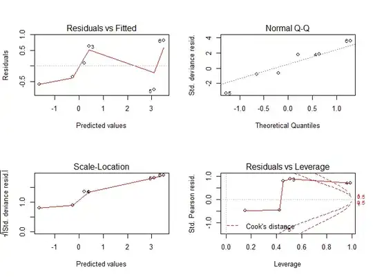
The major concern is that the model is not valid unless the error in (y/x) is Normal with constant variance (or, equivalently, the error in y increases with x). If this is true then we should get a (more or less) linear Q-Q plot, which we do.

One nuance: the interface to the glm logistic model wants two columns for y: "number of successes (S)" and "number of failures (F)". It then calculates the probability as S/(S+F). So we have to provide two columns which mimic this: y and x-y. Then glm(...) will calculate y/(y+(x-y)) = y/x.

Finally, the fit summary suggests that x is important and z may or may not be. You might want to try a model that excludes z and see if that improves AIC.

fit = glm(cbind(y,x-y)~x+z, data=mydata, family=binomial(logit))
summary(fit)
# Call:
# glm(formula = cbind(y, x - y) ~ x + z, family = binomial(logit), 
#     data = mydata)

# Deviance Residuals: 
#        1         2         3         4         5         6  
# -0.59942  -0.35394   0.62705   0.08405  -0.75590   0.81160  

# Coefficients:
#             Estimate Std. Error z value Pr(>|z|)  
# (Intercept)  -2.0264     1.2177  -1.664   0.0961 .
# x             0.6786     0.2695   2.518   0.0118 *
# z            -0.2778     0.1933  -1.437   0.1507  
# ---
# Signif. codes:  0 ‘***’ 0.001 ‘**’ 0.01 ‘*’ 0.05 ‘.’ 0.1 ‘ ’ 1

# (Dispersion parameter for binomial family taken to be 1)

#     Null deviance: 13.7587  on 5  degrees of freedom
# Residual deviance:  2.1149  on 3  degrees of freedom
# AIC: 15.809

par(mfrow=c(2,2))
plot(fit)         # residuals, Q-Q, Scale-Location, and Leverage Plots

mydata$pred <- predict(fit, type="response")
par(mfrow=c(1,1))
plot(mydata$y/mydata$x,mydata$pred,xlim=c(0,1),ylim=c(0,1), xlab="Actual", ylab="Predicted")
abline(0,1, lty=2, col="blue")

jlhoward
  • 58,004
  • 7
  • 97
  • 140
  • I've found also alternatives: `glm(y ~ offset(log(x)) + z, family=poisson(link=log),data=mydata )` or from `library(gamlss)` `gamlss(y/x ~ x + z, data=mydata,family=BEINF)` – ipj Jan 19 '14 at 01:58