R provides Lloyd's algorithm as an option to kmeans(); the default algorithm, by
Hartigan and Wong (1979) is much smarter. Like MacQueen's algorithm (MacQueen, 1967),
it updates the centroids any time a point is moved; it also makes clever (time-saving) choices
in checking for the closest cluster. On the other hand Lloyd's k-means algorithm is the first and simplest of all these clustering algorithms.
Lloyd's algorithm (Lloyd, 1957) takes a set of observations or cases (think: rows of
an nxp matrix, or points in Reals) and clusters them into k groups. It tries to minimize the
within-cluster sum of squares

where u_i is the mean of all the points in cluster S_i. The algorithm proceeds as follows (I'll
spare you the formality of the exhaustive notation):

There is a problem with R's implementation, however, and the problem arises when
considering multiple starting points. I should note that it's generally prudent to consider
several dierent starting points, because the algorithm is guaranteed to converge, but is not
guaranteed to coverge to a global optima. This is particularly true for large, high-dimensional
problems. I'll start with a simple example (large, not particularly dicult).
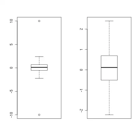
(Here I will paste some images as we can not write mathematical formulaswith latex)


Note that the solution is very similar to the one achieved earlier, although the ordering of the
clusters is arbitrary. More importantly, the job only took 0.199 seconds in parallel! Surely
this is too good to be true: using 3 processor cores should, at best, taken one third of the
time of our first (sequential) run. Is this a problem? It sounds like free lunch. There is no
problem with a free lunch once in a while, is there?
This doesn't always work with R functions, but sometimes we have a chance to look directly
at the code. This is one of those times. I'm going to put this code into file, mykmeans.R,
and edit it by hand, inserting cat() statements in various places. Here's a clever way to do
this, using sink() (although this doesn't seem to work in Sweave, it will work interactively):
> sink("mykmeans.R")
> kmeans
> sink()
Now editing the file, changing the function name and adding cat() statements. Note
that you also have to delete a trailing line: :

We can then repeat our explorations, but using mykmeans():
> source("mykmeans.R")
> start.kmeans <- proc.time()[3]
> ans.kmeans <- mykmeans(x, 4, nstart = 3, iter.max = 10, algorithm = "Lloyd")
JJJ statement 1: 0 elapsed time.
JJJ statement 5: 2.424 elapsed time.
JJJ statement 6: 2.425 elapsed time.
JJJ statement 7: 2.52 elapsed time.
JJJ statement 6: 2.52 elapsed time.
JJJ statement 7: 2.563 elapsed time.
Now we're in business: most of the time was consumed before statement 5 (I knew this of
course, which is why statement 5 was 5 rather than 2)...
You can keep on playing with it
Here is code:
#######################################################################
# kmeans()

N <- 100000
x <- matrix(0, N, 2)
x[seq(1,N,by=4),] <- rnorm(N/2)
x[seq(2,N,by=4),] <- rnorm(N/2, 3, 1)
x[seq(3,N,by=4),] <- rnorm(N/2, -3, 1)
x[seq(4,N,by=4),1] <- rnorm(N/4, 2, 1)
x[seq(4,N,by=4),2] <- rnorm(N/4, -2.5, 1)
start.kmeans <- proc.time()[3]
ans.kmeans <- kmeans(x, 4, nstart=3, iter.max=10, algorithm="Lloyd")
ans.kmeans$centers
end.kmeans <- proc.time()[3]
end.kmeans - start.kmeans

these <- sample(1:nrow(x), 10000)
plot(x[these,1], x[these,2], pch=".")
points(ans.kmeans$centers, pch=19, cex=2, col=1:4)

library(foreach)
library(doMC)
registerDoMC(3)
start.kmeans <- proc.time()[3]
ans.kmeans.par <- foreach(i=1:3) %dopar% {
  return(kmeans(x, 4, nstart=1, iter.max=10, algorithm="Lloyd"))
}
TSS <- sapply(ans.kmeans.par, function(a) return(sum(a$withinss)))
ans.kmeans.par <- ans.kmeans.par[[which.min(TSS)]]
ans.kmeans.par$centers
end.kmeans <- proc.time()[3]
end.kmeans - start.kmeans

sink("mykmeans.Rfake")
kmeans
sink()

source("mykmeans.R")
start.kmeans <- proc.time()[3]
ans.kmeans <- mykmeans(x, 4, nstart=3, iter.max=10, algorithm="Lloyd")
ans.kmeans$centers
end.kmeans <- proc.time()[3]
end.kmeans - start.kmeans

#######################################################################
# Diving

x <- read.csv("Diving2000.csv", header=TRUE, as.is=TRUE)
library(YaleToolkit)
whatis(x)

x[1:14,c(3,6:9)]

meancol <- function(scores) {
  temp <- matrix(scores, length(scores)/7, ncol=7)
  means <- apply(temp, 1, mean)
  ans <- rep(means,7)
  return(ans)
}
x$panelmean <- meancol(x$JScore)

x[1:14,c(3,6:9,11)]

meancol <- function(scores) {
  browser()
  temp <- matrix(scores, length(scores)/7, ncol=7)
  means <- apply(temp, 1, mean)
  ans <- rep(means,7)
  return(ans)
}

x$panelmean <- meancol(x$JScore)
Here is description:
Number of cases: 10,787 scores from 1,541 dives (7 judges score each
dive) performed in four events at the 2000 Olympic Games in Sydney,
Australia.

Number of variables: 10.

Description: A full description and analysis is available in an
article in The American Statistician (publication details to be
announced).

Variables:

Event       Four events, men's and women's 3M and 10m.
Round       Preliminary, semifinal, and final rounds.
Diver       The name of the diver.
Country     The country of the diver.
Rank        The final rank of the diver in the event.
DiveNo      The number of the dive in sequence within round.
Difficulty  The degree of difficulty of the dive.
JScore      The score provided for the judge on this dive.
Judge       The name of the judge.
JCountry    The country of the judge.
And dataset to experiment with it https://www.dropbox.com/s/urgzagv0a22114n/Diving2000.csv