4

I have a data of protein-protein interactions in a data frame entitled: s1m. Each DB and AD pair make an interaction and I can plot it as well:

> head(s1m)
     DB_num AD_num
[1,]      2   8153
[2,]      7   3553
[3,]      8   4812
[4,]     13   7838
[5,]     24   3315
[6,]     24   6012

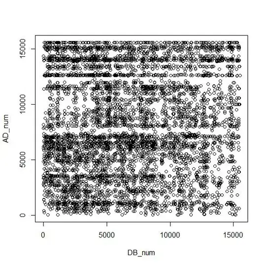
Plot of the data looks like: http://i.imgur.com/RTaeJ5r.jpg

I then used code I found on this site to plot filled contour lines:

## compute 2D kernel density, see MASS book, pp. 130-131
require(MASS)
z <- kde2d(s1m[,1], s1m[,2], n=50)
plot(s1m, xlab="X label", ylab="Y label", pch=19, cex=.4)
filled.contour(z, drawlabels=FALSE, add=TRUE)

It gave me the resulting image(minus the scribbles): result

MY QUESTION: I need to annotate each line of data in the original s1m data frame with a number corresponding to its height on the contour map (hence my scribbles on the image above). I think the list z has the values I am looking for, but I am not sure.

In the end I would want my data to hopefully look something like this so I could study the protein interactions in groups:

         DB_num AD_num   height
    [1,]      2   8153        1
    [2,]      7   3553        1
    [3,]      8   4812        3
    [4,]     13   7838        6
    [5,]     24   3315        2
    [6,]     24   6012        etc.
Drew Steen
  • 16,045
  • 12
  • 62
  • 90
  • 1
    When you attach the value 1, 2, 3, etc to each combination of `DB_num` and `AD_num` are those dummy numbers referring to the actual density or the bin into which it's density falls. In other words, is 2 on your plot referring to the actual value 2 or to the 2nd bin (which takes values 1e-9 to 1.5e9? – Gavin Simpson Jul 22 '13 at 19:57
  • 1
    Since `contour.plot` seems not to return useful values, I suppose this involves two issues that are a bit tricky: (i) mapping from the values in `s1m` to the lattice-like coordinates used by the contour plot, and (ii) reproducing the levels assigned in the different positions of the grid; granted, that is some kind of bricolage, but (ii) can maybe be achieved by borrowing and invoking `contour.plot`'s own syntax, e.g. `levels <- cut(as.numeric(z$z),pretty(range(z$z),20))`, or computing levels yourself and setting the corresponding parameter explicitly... – texb Jul 22 '13 at 20:20
  • @GavinSimpson The dummy numbers would be referring to the bin, but the having the actual values of the points would probably work too. – Kerpal Jenkiens Jul 22 '13 at 20:33
  • Maybe what you need is contour lines? http://www.r-bloggers.com/fix-overplotting-with-colored-contour-lines/ – Roman Luštrik Jul 22 '13 at 20:37
  • @texb - I'm not sure what you mean. I just started using R. How would I match the values in the grid (stored in 'levels' I think) to the individual points? Or how would I compute the "density" of each point explicitly? – Kerpal Jenkiens Jul 22 '13 at 20:51
  • @Roman Luštrik The graph produced is fine, I need the data that goes along with the graph annotated to the points. Is there some way to match the points with the 'height' of the contour line they are in? – Kerpal Jenkiens Jul 22 '13 at 20:51
  • @KerpalJenkiens OK, thanks for confirmation. I've added something now which should get you 99.9% of the way there. – Gavin Simpson Jul 22 '13 at 20:52
  • @texb +1 you are pretty much there, only missing thing is to point to the component `z` of the object returned by `kde2d()` to give the actual `heights` used in the plot, *before grouping*. – Gavin Simpson Jul 22 '13 at 20:54
  • @KerpalJenkiens I missed the need to work with the actual data, not the points the KDE was evaluated at. – Gavin Simpson Jul 22 '13 at 21:37

1 Answers1

3

This is one option if you want the actual height not the bin each is assigned to

## dummy data
DF <- data.frame(DB_num = rnorm(10000), AD_num = rnorm(10000))

require("MASS")

kde <- kde2d(DF[,1], DF[,2], n = 50)

Note the kde2d returns as component z which is a matrix with (in this case) 50 rows and columns where rows correspond to the x data and columns to the y data. As a matrix is just a vector, and the data are filled by columns, we can exploit this and stack the x and y values n times each (n = 50 here), then unwind kde$z

dd <- dim(kde$z)
res <- data.frame(DB_num = rep(kde$x, times = dd[1]),
                  AD_num = rep(kde$y, times = dd[2]),
                  height = as.numeric(kde$z))

This produces

> head(res)
        DB_num      AD_num                                  height
1 -3.582508378 -3.79074271 0.0000000000000000000000000006907447484
2 -3.429230262 -3.63682706 0.0000000000000000000000002951259863229
3 -3.275952146 -3.48291141 0.0000000000000000000000558203373144190
4 -3.122674029 -3.32899576 0.0000000000000000000055565720524140235
5 -2.969395913 -3.17508011 0.0000000000000000014967010810961022503
6 -2.816117797 -3.02116446 0.0000000000000008159370528768207499471

To get the bins, you'd need to follow what filled.contour did, which is to form breaks via

nlevels <- 20 ## default
brks <- pretty(range(res$height), nlevels)

> brks
 [1] 0.00 0.01 0.02 0.03 0.04 0.05 0.06 0.07 0.08 0.09 0.10 0.11 0.12 0.13 0.14
[16] 0.15 0.16

Then use cut to assign each height to a bin on basis of brks, something like

res <- transform(res, bin = as.numeric(cut(height, brks)))

Which gives

> head(res)
        DB_num      AD_num                                  height bin
1 -3.582508378 -3.79074271 0.0000000000000000000000000006907447484   1
2 -3.429230262 -3.63682706 0.0000000000000000000000002951259863229   1
3 -3.275952146 -3.48291141 0.0000000000000000000000558203373144190   1
4 -3.122674029 -3.32899576 0.0000000000000000000055565720524140235   1
5 -2.969395913 -3.17508011 0.0000000000000000014967010810961022503   1
6 -2.816117797 -3.02116446 0.0000000000000008159370528768207499471   1

You'll probably want to check the details of ?cut to determine behaviour on the boundary of a bin, but that should get you close enough.

Gavin Simpson
  • 170,508
  • 25
  • 396
  • 453
  • @texb I don't think that is going to work well. It would be better to use a tool that returned enough things to allow for predictions at the actual values observed. I think something in the **kernsmooth** package would be ideal. Let me look. (and yes, I missed the line about wanting to tie each observation in the original data). – Gavin Simpson Jul 22 '13 at 21:31
  • Actually, scratch that, **KernSmooth** does exactly the same as `kde2d()` with its function `bkde2D()` – Gavin Simpson Jul 22 '13 at 21:34
  • @texb In lieu of that, I think your addition is probably the easiest thing to do at this stage. +1 – Gavin Simpson Jul 22 '13 at 21:38
  • First of all, very clever answers, but @textb I tried using your method and I am not sure that it is placing the points into accurate bins. Using a random set of points, I used the Gavin's method and annotated the DF list. I then looked at where some of the points were falling by eye, and some seemed off. I didn't know how to markup the filled.contour graphic so I made another one for proof of concept. I don't the point marked by the lines should be in that high of a bin: http://i.imgur.com/63H9RZC.png – Kerpal Jenkiens Jul 22 '13 at 22:34
  • @KerpalJenkiens The real issue is that you want something to predict the `height` as you would be reading off the plot, when neither `kde2d` nor `filled.contour` allow this. `kde2d` is just evaluating the density at 50x50 evenly spaced locations and `filled.contour` is finding contours and filling the regions between them. I'm looking for a 2D KDE that will return estimates of the density at the observed values. It would be best to use such a thing, assuming it exists! – Gavin Simpson Jul 22 '13 at 22:38
  • @KerpalJenkiens: There is certainly an element of tinkering about it; maybe one useful intermediate step would be to (graphically) ensure that the identification of the nearest grid elements works as intended (e.g. like `mat <- expand.grid((s <- seq(0,1,.2)),s); image(outer(s,s,"^")); new.obs <- data.frame(runif(8),runif(8)); nearest <- apply(new.obs,1,function(x) which.min((x[1]-mat[,1])**2+(x[2]-mat[,2])**2)); arrows(new.obs[,1],new.obs[,2],mat[nearest,1],mat[nearest,2])`), and potentially querying the folks at [stats.stackexchange.com] about the general approach might also be an idea. – texb Jul 22 '13 at 23:25
  • @KerpalJenkins: I had to delete my original comment about complementing `s1m` with with some meaningful density estimate 'in the vicinity' of the observation, because it seemed to contain some faulty bracketing (which probably produced the errors shown in your graphic); sorry. I hope this works better: `which.min.d <- function(x1,y1,x2,y2) which.min((x1-x2)**2+(y1-y2)**2); DF$height <- apply(DF,1,function(x) res[which.min.d(x[1],x[2],res$DB_num,res$AD_num),"height"])`, but still recommend visualizing results e.g. by using `arrows` as demonstrated above... – texb Jul 23 '13 at 08:43
  • Okay, I've tried using the approach listed in the original answer by @GavinSimpson, and it seems that the bins listed in `res` do not match up when I checked a few by hand. Therefore, I am guessing that trying to annotate `DF` would be futile if `res` is wrong. It was a noble attempt, but if it cannot be done, it's alright since my research has shifted to a different method anyway. – Kerpal Jenkiens Jul 24 '13 at 19:24
  • not sure if `res <- data.frame(DB_num = rep(kde$x, times = dd[1]), AD_num = rep(kde$y, times = dd[2]), etc` is correct here - you're just repeating every coordinate 50 times. I think it should be that the y coordinates need to be repeated with `each = ...`: `data.frame(DB_num = rep(kde$x, times = dd[1]), AD_num = rep(kde$y, each = dd[2]), ...)` – tjebo Apr 05 '20 at 11:43