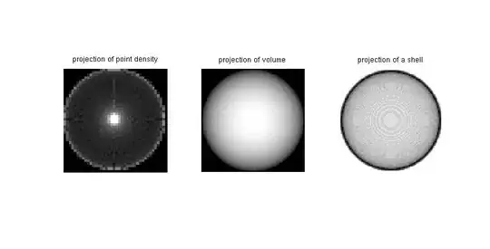
It is possible that I completely misunderstand your question, in which case I apologize; but I think one of the following three methods may in fact be what you need. Note that method 3 gives an image that looks a lot like the example you provided... but I got there with a very different route (not using the sphere command at all, but computing "voxels inside" and "voxels outside" by working directly with their distance from the center). I inverted the second image compared to the third on since it looked better that way - filling the sphere with zeros made it look almost like a black disk.
%% method 1: find the coordinates, and histogram them
[x y z]=sphere(200);
xv = linspace(-1,1,40);
[xh xc]=histc(x(:), xv);
[yh yc]=histc(y(:), xv);

% sum the occurrences of coordinates using sparse:
sm = sparse(xc, yc, ones(size(xc)));
sf = full(sm);

figure;
subplot(1,3,1);
imagesc(sf); axis image; axis off
caxis([0 sf(19,19)]) % add some clipping
title 'projection of point density'

%% method 2: fill a sphere and add its volume elements:
xv = linspace(-1,1,100);
[xx yy zz]=meshgrid(xv,xv,xv);
rr = sqrt(xx.^2 + yy.^2 + zz.^2);
vol = zeros(numel(xv)*[1 1 1]);
vol(rr<1)=1;
proj = sum(vol,3);
subplot(1,3,2)
imagesc(proj); axis image; axis off; colormap gray
title 'projection of volume'

%% method 3: visualize just a thin shell:
vol2 = ones(numel(xv)*[1 1 1]);
vol2(rr<1) = 0;
vol2(rr<0.95)=1;
projShell = sum(vol2,3);
subplot(1,3,3);
imagesc(projShell); axis image; axis off; colormap gray
title 'projection of a shell'