1

I've used fitdistr function from R MASS package to adjust a Weibull 2 parameters probability density function (pdf).

This is my code:

require(MASS)

h = c(31.194, 31.424, 31.253, 25.349, 24.535, 25.562, 29.486, 25.680, 26.079, 30.556,      30.552, 30.412, 29.344, 26.072, 28.777, 30.204, 29.677, 29.853, 29.718, 27.860, 28.919, 30.226, 25.937, 30.594, 30.614, 29.106, 15.208, 30.993, 32.075, 31.097, 32.073, 29.600, 29.031, 31.033, 30.412, 30.839, 31.121, 24.802, 29.181, 30.136, 25.464, 28.302, 26.018, 26.263, 25.603, 30.857, 25.693, 31.504, 30.378, 31.403, 28.684, 30.655,  5.933, 31.099, 29.417, 29.444, 19.785, 29.416, 5.682, 28.707, 28.450, 28.961, 26.694, 26.625, 30.568, 28.910, 25.170, 25.816, 25.820)

weib = fitdistr(na.omit(h),densfun=dweibull,start=list(scale=1,shape=5))

hist(h, prob=TRUE, main = "", xlab = "x", ylab = "y", xlim = c(0,40), breaks = seq(0,40,5))
curve(dweibull(x, scale=weib$estimate[1], shape=weib$estimate[2]),from=0, to=40, add=TRUE)

Now, I would like to create the Weibull cumulative distribution function (cdf) and plot it as a graph:

enter image description here
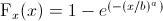
, where x > 0, b = scale , a = shape

I tried to apply scale and shape parameters for h using the formula above, but it was not this way.

Andre Silva
  • 4,782
  • 9
  • 52
  • 65

2 Answers2

5

Here's a stab at a cumulative density function. You just have to remember to include an adjustment for the spacing of the sampling points (note: it works for sampling points with uniform spacing less than or equal to 1):

cdweibull <- function(x, shape, scale, log = FALSE){
  dd <- dweibull(x, shape= shape, scale = scale, log = log)
  dd <- cumsum(dd) * c(0, diff(x))
  return(dd)
}

The discussion above about scale differences notwithstanding, you can plot it over your graph the same as dweibull:

require(MASS)

h = c(31.194, 31.424, 31.253, 25.349, 24.535, 25.562, 29.486, 25.680,
      26.079, 30.556, 30.552, 30.412, 29.344, 26.072, 28.777, 30.204, 
      29.677, 29.853, 29.718, 27.860, 28.919, 30.226, 25.937, 30.594, 
      30.614, 29.106, 15.208, 30.993, 32.075, 31.097, 32.073, 29.600, 
      29.031, 31.033, 30.412, 30.839, 31.121, 24.802, 29.181, 30.136, 
      25.464, 28.302, 26.018, 26.263, 25.603, 30.857, 25.693, 31.504, 
      30.378, 31.403, 28.684, 30.655,  5.933, 31.099, 29.417, 29.444, 
      19.785, 29.416, 5.682, 28.707, 28.450,  28.961, 26.694, 26.625, 
      30.568, 28.910, 25.170, 25.816, 25.820)

weib = fitdistr(na.omit(h),densfun=dweibull,start=list(scale=1,shape=5))

hist(h, prob=TRUE, main = "", xlab = "x", 
     ylab = "y", xlim = c(0,40), breaks = seq(0,40,5), ylim = c(0,1))

curve(cdweibull(x, scale=weib$estimate[1], shape=weib$estimate[2]),
  from=0, to=40, add=TRUE)

histogram with weibull cumulative density overlay

Noah
  • 1,404
  • 8
  • 12
  • It may work for sampling points with a uniform spacing greater than one, but the plot is understandably less pretty. – Noah Apr 18 '13 at 21:47
  • That is great! Just one doubt. The adjustment you talked about is in the `lag` argument inside of `diff(x)`? For example: default for `lag` is 1, but if my sample had larger spacing I would setup lag = 2,4,10,etc.... Is that it? – Andre Silva Apr 18 '13 at 23:08
  • Andre, I don't think so, because `cumsum` is working directly on the results that are returned by `dweibull`. The 'lag' correction, in a sense, is _what_ is returned by `diff`. You can try it: After running the `hist` command above, run `lines(seq(0, 40, by = 4), cdweibull(seq(0, 40, by = 4), scale=weib$estimate[1], shape=weib$estimate[2]))`. You'll see that a line gets added, but it's rougher, because the resolution is much lower. – Noah Apr 19 '13 at 00:03
  • In other words, it should be fine, even with a larger sampling spacing, provided that the spacing is uniform. – Noah Apr 19 '13 at 00:05
  • Awesome!! Thank's a lot Noah. – Andre Silva Apr 19 '13 at 00:08
4

This works for my data but yours may differ. It uses rweibull3 function from FAdist package.

>h=rweibull3(1000,2,2,2)

>#this gives some warnings...that I ignore.
>weib = fitdistr(h,densfun=dweibull3,start=list(scale=1,shape=5,thres=0.5))

There were 19 warnings (use warnings() to see them)    

The thing to be aware of is that the start values effect the way the fit proceeds. So if the start values are close to the true values, you will get fewer warnings.

>curve(dweibull3(   x, 
            scale=weib$estimate[1], 
            shape=weib$estimate[2], 
            thres=weib$estimate[3]),
            add=TRUE)

enter image description here

agenis
  • 8,069
  • 5
  • 53
  • 102
Seth
  • 4,745
  • 23
  • 27
  • Is the weibull density defined for the range of values you want to fit? It doesnt work for values zero or less. – Seth Mar 12 '13 at 21:21