18

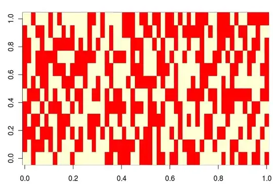
I am hoping to construct some charts to display the shooting tendencies/effectiveness of some NBA players and teams. I would like to format the hexagons as follows: size will represent the number of shots and color will represent the relative efficiency (pts/attempt) from that location. Here is a great example of what I'm looking for, created by Kirk Goldsberry:

Ray Allen, by Kirk Goldsberry

I have been able to use hexbins and hexTapply to achieve something close to the desired result, but the shapes are circles. Here is my code (which includes sample data):

library(hexbin); library(ggplot2)
df <- read.table(text="xCoord yCoord   pts
11.4     14.9     2
2.6       1.1      0
4.8       4.1      2
-14.4    8.2      2
4.2       0.3      0
0.4       0.0     2
-23.2   -1.1      3", header=TRUE)
h <- hexbin (x=df$xCoord, y = df$yCoord, IDs = TRUE, xbins=50)
pts.binned <- hexTapply (h, df$pts, FUN=mean)

df.binned <- data.frame (xCoord  = h@xcm, 
          yCoord  = h@ycm, FGA = h@count, pts = pts.binned)

chart.player <- ggplot (df.binned, aes (x =xCoord , 
                  y =yCoord , col = pts, size = FGA)) + coord_fixed() + 
geom_point()  + scale_colour_gradient("Points/Attempt", low = "green", high="red")

Another way to think about it would be to coloring the hexagons in plot(h, style="lattice") by pts/attempt -- but I'm not sure how to do that, either.

Is there a way to get this graph with hexagons rather than circles?

Jason Sundram
  • 12,225
  • 19
  • 71
  • 86
Wynnerbago
  • 181
  • 4
  • Just I am curious. what is the meaning of negative coordinates here? The point is counted in basket even when you shoot outside the ground? – agstudy Feb 12 '13 at 19:48
  • I think the basket's location is c(0,0). – IRTFM Feb 12 '13 at 19:57
  • That's correct DWin. The coordinates are in feet and are relative to the basket at 0,0. So the shot taken at (-23.2, -1.1) would be a left corner 3 pointer that is 23.2 feet to the left of the hoop and almost a foot behind the center of the hoop. Note that the hoop is 5.25 feet from the baseline, so this shot is still in the field of play. Thanks for the edits DWin – Wynnerbago Feb 12 '13 at 20:02
  • Have you tried using [`stat_binhex`](http://docs.ggplot2.org/0.9.3/stat_binhex.html) from ggplot2? – mitchus Feb 12 '13 at 20:21
  • I have tried stat_binhex and I haven't been able to get it to work, but if you have a suggested syntax, I would love to try it – Wynnerbago Feb 12 '13 at 20:38
  • I wonder if shot success failure would be better than points per attempt. I say that becuase the 3 point line is going to show an obvious tendency to higher points but it could be misleading if the player only makes the shot 50% of the time. – Brandon Bertelsen Feb 13 '13 at 02:02
  • Actually, looking at it more closely, using `stat_binhex` you can't really show two features (frequency and accuracy) at once. The sizes of the tiles are the same for the entire surface. – mitchus Feb 13 '13 at 10:24
  • @Brandon -- If the chart is trying to show "expected value" of a shot from a certain location, I think its a good idea to use the pts/attempt metric over shooting percentage. – Wynnerbago Feb 13 '13 at 18:45

1 Answers1

9

First thank you for this question and for sharing this plot with great imagination!

Here a attempt using lattice package. Mainly I implement you idea of : coloring the hexagons in plot(h, style="lattice") by pts/attempt". The use of lattice is also motivated by the fact that you can use grid functions within the lattice panel functions( to draw the ground details for example)

I generate some data

dat <- data.frame(
  xCoord = round(runif(1000,-30,30),2),
  yCoord = round(runif(1000,-2,30),2),
  pts = sample(c(0,2,3),100,rep=T))
#dat$pts[dat$xCoord <0 & dat$yCoord] <- 3

here the plot:

    xyplot(yCoord~xCoord,data =dat , panel = function(x,y,...)
   {
     hbin<-hexbin(dat$xCoord,dat$yCoord,xbins=50,IDs=TRUE)
     mtrans<-hexTapply(hbin,dat$pts,sum,na.rm=TRUE)
     cols <- rainbow( 4,alpha=0.5)
     grid.hexagons(hbin, style='lattice',
                   ,minarea=0.5,maxarea=5,colorcut=c(0,.6,1),
                   border=NA,
                   pen=cols[mtrans+1])
     ## Now you can get fun to draw the ground here
     ## something like...
     ## grid.circle(gp=gpar(fill=NA))
   })

enter image description here

EDIT Using OP real data. I get this plot. You need to play with minarea and ``maxareaargument to define overlapping regions. I add also an image as abckground usinggrid.raster`. I don't have plot skills so I choose one from he net, but you can use this technique to add a ground. I am sure you can do a better image.

library(lattice)
library(hexbin)
library(png)
xyplot(locationY~locationX,data =dat , panel = function(x,y,...)
{
    ## imgae bakground
    m <- readPNG('basket.png')
    rimg <- as.raster(m)
    grid.raster(rimg, x=0, y=61.5, just="top", width=50,
              default.units = "native")
    panel.fill(col=rgb(1,1,1,alpha=0.8))

    hbin<-hexbin(dat$locationX,dat$locationY,xbins=50,IDs=TRUE)
    mtrans<-hexTapply(hbin,dat$Points,sum,na.rm=TRUE)
    cols <- rainbow(4)
    grid.hexagons(hbin, style='lattice',
                  ,minarea=0.1,maxarea=50,colorcut=c(0,.6,1),
                  border=NA,
                  pen=cols[mtrans+1])
})

enter image description here

agstudy
  • 119,832
  • 17
  • 199
  • 261
  • Thanks agstudy! I will try this out today and let you know how it goes. – Wynnerbago Feb 13 '13 at 18:46
  • I was using `geom_path` to draw the "court lines". For example, I was using the following code to draw curved portion of the 3 point line: `arcX2<-seq(length=5000, from=-22, to=22) arcY2<-sqrt(23.75^2-arcX2^2) arc2data <- data.frame(x=arcX2,y=arcY2) arctwo<-geom_path(data=arc2data , aes(arcX2,arcY2), colour="grey", size=1)` Can I use the `grid` functions to do something similar? – Wynnerbago Feb 13 '13 at 21:44
  • @Wynnerbago did you try at least this on real data? for your second comment you have a ggplot2 plot and you would to convert it to lattice plot? is'ntit? – agstudy Feb 14 '13 at 01:24
  • Yes and if there is a good way for me to upload a larger sample I would be happy to. Yes, they are ggplot2 functions. Being very new to R programming, I am kind of picking this all up as I go along. My first attempt at this was using ggplot2. Going of your suggestion, I was trying the grid.hexagon route. I was just curious if I could convert ggplot2 or find an analogous function for drawing in the court lines – Wynnerbago Feb 14 '13 at 01:38
  • What do you mean by uploading larger sample? You can use something like dropbox to put you sample file then give the link to it in the comment here. I will update my question using it| Yes you can convert ggplot2 to 'lattice'. Note here my solution use grid just because for your particular need(multivariate hexbin) but it is essentially a lattice solution. Hope it is clear. – agstudy Feb 14 '13 at 01:44
  • Here is a copy of some real shot data (http://dl.dropbox.com/u/55588895/shot%20chart%20sample.csv). I am still unclear about a lattice solution vs a ggplot2 solution, but perhaps it will become clear in your update. Thanks again for all your help. – Wynnerbago Feb 14 '13 at 01:59