From Wikipedia:
The percentile rank of a score is the percentage of scores in its frequency distribution that are the same or lower than it.
In order to illustrate this, let's create a distribution, say, a normal distribution, with mean=2 and sd=2, so that we can test (our code) later.
# 1000 samples from normal(2,2)
x1 <- rnorm(1000, mean=2, sd=2)
Now, let's take the same percentile rank you've mentioned in your post. Let's divide it by 100 so that they represent cumulative probabilities.
cum.p <- c(1, 7, 12, 23, 41, 62, 73, 80, 92, 99)/100
And what are the values (scores) corresponding to these percentiles?
# generating values similar to your x.
x <- c(t(quantile(x1, cum.p)))
> x
 [1] -2.1870396 -1.4707273 -1.1535935 -0.8265444 -0.2888791
         0.2781699  0.5893503  0.8396868  1.4222489  2.1519328
This means that 1% of the data is lesser than -2.18. 7% of the data is lesser than -1.47 etc... Now, we have the x and cum.p (equivalent to your PercRank). Let's forget x1 and the fact that this should be a normal distribution. To find out what distribution it could be, let's get actual probabilities from the cumulative probabilities by using diff that takes the difference between nth and (n-1)th element.
prob <- c( cum.p[1], diff(cum.p), .01)
> prob
# [1] 0.01 0.06 0.05 0.11 0.18 0.21 0.11 0.07 0.12 0.07 0.01
Now, all we have to do is is to generate samples of size, say, 100 (could be any number), for each interval of x (x[1]:x[2], x[2]:x[3] ...) and then finally sample from this huge data as many number of points as you need (say, 10000), with probabilities mentioned above.
This can be done by:
freq <- 10000 # final output size that we want

# Extreme values beyond x (to sample)
init <- -(abs(min(x)) + 5)
fin  <- abs(max(x)) + 5

ival <- c(init, x, fin) # generate the sequence to take pairs from
len <- 100 # sequence of each pair

s <- sapply(2:length(ival), function(i) {
    seq(ival[i-1], ival[i], length.out=len)
})
# sample from s, total of 10000 values with probabilities calculated above
out <- sample(s, freq, prob=rep(prob, each=len), replace = T)
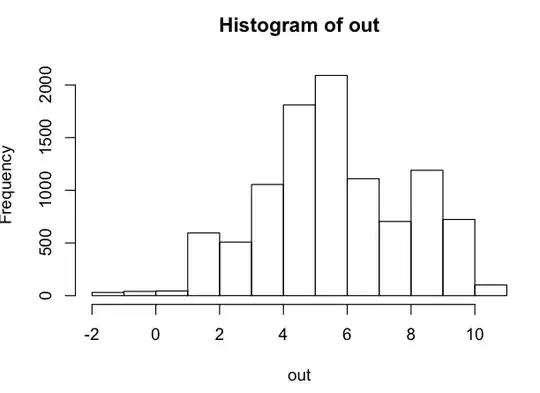
Now, we have 10000 samples from the distribution. Let's look at how it is. It should resemble a normal distribution with mean = 2 and sd = 2.
> hist(out)
> c(mean(out), sd(out))
# [1] 1.954834 2.170683
It is a normal distribution (from the histogram) with mean = 1.95 and sd = 2.17 (~ 2).
Note: Some things what I've explained may have been roundabout and/or the code "may/may not" work with some other distributions. The point of this post was just to explain the concept with a simple example.
Edit: In an attempt to clarify @Dwin's point, I tried the same code with x = 1:10 corresponding to OP's question, with the same code by replacing the value of x.
cum.p <- c(1, 7, 12, 23, 41, 62, 73, 80, 92, 99)/100
prob <- c( cum.p[1], diff(cum.p), .01)
x <- 1:10

freq <- 10000 # final output size that we want

# Extreme values beyond x (to sample)
init <- -(abs(min(x)) + 1)
fin  <- abs(max(x)) + 1

ival <- c(init, x, fin) # generate the sequence to take pairs from
len <- 100 # sequence of each pair

s <- sapply(2:length(ival), function(i) {
    seq(ival[i-1], ival[i], length.out=len)
})
# sample from s, total of 10000 values with probabilities calculated above
out <- sample(s, freq, prob=rep(prob, each=len), replace = T)

> quantile(out, cum.p) # ~ => x = 1:10
# 1%     7%    12%    23%    41%    62%    73%    80%    92%    99%
# 0.878  1.989  2.989  4.020  5.010  6.030  7.030  8.020  9.050 10.010

> hist(out)