Solve non-linear non homogeneous differential equation with python (Duffing oscillator)

Question

I try to solve the Duffing equation using odeint:

def func(z, t):
    q, p = z
    return [p, F*np.cos(OMEGA * t) + Fm*np.cos(3*OMEGA * t) + 2*gamma*omega*p - omega**2 * q - beta * q**3]
OMEGA = 1.4
T = 1 / OMEGA
F = 0.2
gamma = 0.1
omega = -1.0
beta = 0.0
Fm = 0

z0 = [1, 0]

psi = 1 / ((omega**2 - OMEGA**2)**2 + 4*gamma**2*OMEGA**2)
wf = np.sqrt(omega**2 - gamma**2)

t = np.linspace(0, 100, 1000)
sol1 = odeintw(func, z0, t, atol=1e-13, rtol=1e-13, mxstep=1000)

When F = gamma = beta = 0 we have a system of two linear homogeneous equations. It's simple!

But when F not equal 0 the system becomes non homogeneous. The problem is that the numerical solution does not coincide with the analytical one:

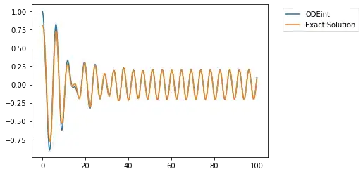
^{Figure 1}

the numerical solution does not take into account the inhomogeneous solution of the equation.

I have not been able to figure out if it is possible to use here solve_bvp function. Could you help me?

The exact solution is obviously wrong, it does not start at the value `1`. — Lutz Lehmann, Jan 24 '21 at 19:53
@LutzLehmann, I am looking for the general solution as the sum of the solution of a homogeneous equation and a particular non homogeneous: X(t) + Xnon(t). It does start at value 1 if there is external force (F = 0), if F is not equal to zero, then the force contributes from the start. Am I wrong? — Andrew Semyonov, Jan 24 '21 at 20:07
If the position at time zero is 1, then any force will not change it. You have to adapt the coefficients of the homogeneous solution to fit. (WolframAlpha makes a huge mess of the exact solution.) — Lutz Lehmann, Jan 24 '21 at 20:10
This was just a comment about a readily available CAS. But it shows that sometimes the manual solution is more straightforward. — Lutz Lehmann, Jan 24 '21 at 20:30

score 0 · Accepted Answer · answered Jan 24 '21 at 21:01

Inserting the constants, the equation becomes

x'' + 2*c*x' + x = F*cos(W*t)

The general solution form is

x(t)=A*cos(W*t)+B*sin(W*t)+exp(-c*t)*(C*cos(w*t)+D*sin(w*t))

w^2=1-c^2

for the particular solution one gets

  -W^2*(A*cos(W*t)+B*sin(W*t))
+2*c*W*(B*cos(W*t)-A*sin(W*t))
+     (A*cos(W*t)+B*sin(W*t))
=F*cos(W*t)

 (1-W^2)*A + 2*c*W*B = F
-2*c*W*A + (1-W^2)*B = 0

For the initial conditions it is needed that

A+C = 1
W*B-c*C+w*D=0

In python code thus

F=0.2; c=0.1; W=1.4
w=(1-c*c)**0.5

A,B = np.linalg.solve([[1-W*W, 2*c*W],[-2*c*W,1-W*W]], [F,0])
C = 1-A; D = (c*C-W*B)/w

print(f"w={w}, A={A}, B={B}, C={C}, D={D}")

with the output

w=0.99498743710662, A=-0.192, B=0.056, C=1.192, D=0.04100554286257586

continuing

t = np.linspace(0, 100, 1000)
u=odeint(lambda u,t:[u[1], F*np.cos(W*t)-2*c*u[1]-u[0]], [1,0],t, atol=1e-13, rtol=1e-13)
plt.plot(t,u[:,0],label="odeint", lw=3); 
plt.plot(t,A*np.cos(W*t)+B*np.sin(W*t)+np.exp(-c*t)*(C*np.cos(w*t)+D*np.sin(w*t)), label="exact"); 
plt.legend(); plt.grid(); plt.show();

results in an exact fit

Thanks! I've already done it. My solution coincided with yours. — Andrew Semyonov, Jan 25 '21 at 09:05

Solve non-linear non homogeneous differential equation with python (Duffing oscillator)

1 Answers1