Efficiently and accurately interpolate between finite-element node stress points in python

Question

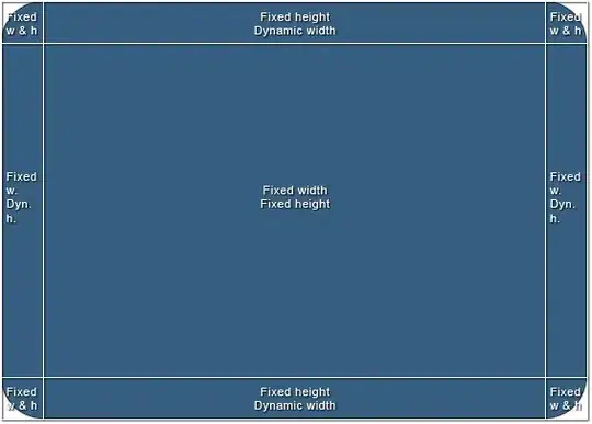
I'd like to interpolate some 3D finite-element stress field data from a bunch of known nodes at points where nodes don't exist. I realise that node stresses are already extrapolated from gauss points, but it is the best I can do with the data I have available. The image below gives a 2D representation. The red and pink points would represent locations where I'd like to interpolate the value.

Initially I thought I could find the smallest bounding box (hull) or simplex that contained the point of interest and no other known points. Visualising this in 2D I realised that this might lead to ignoring data from a close-by value, incorrectly. I was planning on using the scipy LindearNDInterpolator but I notice there is some unexpected behaviour, and I'm worried it will exclude nearby points in the way that I just described. Notice how the pink point would not reference from the green triangle but ignore the point outside the orange triangle, although it is probably more relevant.

As far as I can tell the best way is to take the nearest surrounding nodes, and interpolating by weighted averaging on distance. I'm not sure if there is something readily available or if it needs to be written. I'd imagine this is a fairly common problem so I'd presume the wheel has already been invented...

Actually my final goal is to interpolate/regress values for a 3D line through the set of points.

Are radial basis functions a better alternative? – Not a chance Mar 31 '16 at 12:43 — Not a chance, Mar 31 '16 at 12:43

score 1 · Answer 1 · answered Mar 31 '16 at 15:17

You can try Inverse distance weighting. Here is an example in 1D (easily generalizable to 3D):

from pylab import *
# imaginary samples
xmax=10
Npoints=10
x=0.1*randint(0,10*xmax,Npoints)
y=sin(2*x)+x
plot(x,y,ls="",marker="x",color="red",label="samples",ms=9,mew=2)
# interpolation 
x2=linspace(0,xmax,150) # new sampling
def weight(x,x0,p): # modify this function in 3D
    return 1/(((x-x0)**2)**(p/2)+0.00001) # 0.00001 to avoid infinity
y2=zeros_like(x2)
for p in range(1,4):
    for i in range(len(y2)):
        y2[i]=sum(y*weight(x,x2[i],p))/sum(weight(x,x2[i],p))
    plot(x2,y2,label="Interpolation p="+str(p))
legend(loc=2)
show()

Here is the result

As you can see, it's not really fantastic. The best results are, I think, for p=2, but it will be different in 3D. I have obtained better curves with a gaussian weight, but have no theorical background for such a choice.

Thanks for this. Actually I'm worried about using it for work that could impact safety of equipment. I'll look at radial basis functions and see what I can come up with. — Not a chance, May 10 '16 at 14:42

score 0 · Accepted Answer · edited May 23 '17 at 12:30

https://stackoverflow.com/a/36337428/2372254

The first answer here was helpful but the 1-D example shows that the approach actually does some strange things with p=1 (wildy different from the data) and with p=3 we get some weird plateaux.

I took a look at Radial Basis Functions which are implemented in SciPy, and modified JPG's code as follows.

Modified Code

from pylab import *
from scipy.interpolate import Rbf, InterpolatedUnivariateSpline
# imaginary samples
xmax=10
Npoints=10
x=0.1*randint(0,10*xmax,Npoints)

Rbf requires sorted lists:

x.sort()
y=sin(2*x)+x
plot(x,y,ls="",marker="x",color="red",label="samples",ms=9,mew=2)
# interpolation 
x2=linspace(0,xmax,150) # new sampling
def weight(x,x0,p): # modify this function in 3D
    return 1/(((x-x0)**2)**(p/2)+0.00001) # 0.00001 to avoid infinity
y2=zeros_like(x2)
for p in range(1,4):
    for i in range(len(y2)):
        y2[i]=sum(y*weight(x,x2[i],p))/sum(weight(x,x2[i],p))
    plot(x2,y2,label="Interpolation p="+str(p))
yrbf = Rbf(x, y)
fi = yrbf(x2)
plot(x2, fi, label="Radial Basis Function")
ius = InterpolatedUnivariateSpline(x, y)
yius = ius(x2)
plot(x2, yius, label="Univariate Spline")
legend(loc=2)
show()

The results are interesting and probably more suitable to my intended usage. The following figure was produced.

Figure Showing RBF and Univariate Spline example

But the RBF implementation in SciPy (google for alternatives) has a major problem when points are repeated - not likely in a real scenario - and goes completely ballistic:

Figure showing ballistic RBF

When smoothed (smooth=0.1 was used) it goes normal again. This might show some programming weirdness.

Efficiently and accurately interpolate between finite-element node stress points in python

2 Answers2