Cubic spline / curve fitting

Question

I need to determine parameters of Illumintaion change, which is defined by this continuous piece-wise polynomial C(t), where f(t) is is a cubic curve defined by the two boundary points (t1,c) and (t2,0), also f'(t1)=0 and f'(t2)=0. Original Paper: Texture-Consistent Shadow Removal

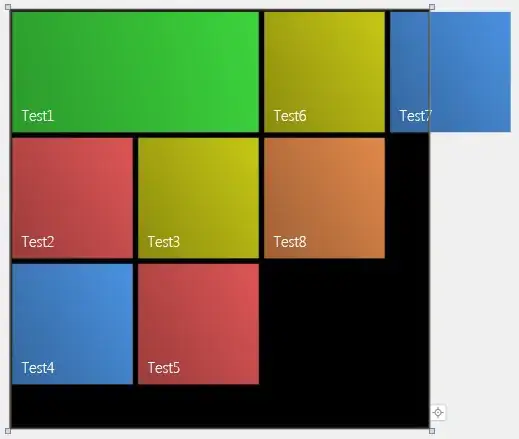
Intensity curve is sampled from the normal on boundary of shadow and it looks like this:

Each row is sample, displaying illumintaion change.So X is number of column and Y is intensity of pixel.

I have my real data like this (one sample avaraged from all samples):

At all I have N samples and I need to determine parameters (c,t1,t2)

How can I do it?

I tried to do it by solving linear equation in Matlab:

avr_curve is average curve, obtained by averaging over all samples.

f(x)= x^3+a2*x^2+a1*x1+a0 is cubic function

%t1,t2 selected by hand
t1= 10;
t2= 15;

offset=10;
avr_curve= [41, 40, 40, 41, 41, 42, 42, 43, 43, 43, 51, 76, 98, 104, 104, 103, 104, 105, 105, 107, 105];
%gradx= convn(avr_curve,[-1 1],'same');

A= zeros(2*offset+1,3);
%b= zeros(2*offset+1,1);
b= avr_curve';
%for i= 1:2*offset+1
for i=t1:t2
  i
  x= i-offset-1
  A(i,1)=  x^2; %a2
  A(i,2)=  x; %a1
  A(i,3)=  1; %a0 
  b(i,1)= b(i,1)-x^3;
end

u= A\b;

figure,plot(avr_curve(t1:t2))


%estimated cubic curve
for i= 1:2*offset+1 
  x= i-offset-1;
  fx(i)=x^3+u(1)*x^2+u(2)*x+u(3);
end

figure,plot(fx(t1:t2))

part of avr_curve on [t1 t2]

cubic curve that I got (don't looks like avr_curve)

so what I'm doing wrong?

UPDATE: Seems my error was due that I model cubic polynomial using 3 variables like this:

f(x)= x^3+a2*x^2+a1*x1+a0 - 3 variables

but then I use 4 variables everything seems ok:

f(x)= a3*x^3+a2*x^2+a1*x1+a0 - 4 variables 

Here is the code in Matlab:

%defined by hand
t1= 10;
t2= 14;

avr_curve= [41, 40, 40, 41, 41, 42, 42, 43, 43, 43, 51, 76, 98, 104, 104, 103, 104, 105, 105, 107, 105];
x=         [1,  2,  3,  4,  5,  6,  7,  8,  9,  10, 11, 12, 13, 14,  15,  16,  17,  18,  19,  20,  21];
%x=        [-10, -9, -8, -7, -6, -5, -4, -3, -2, -1, 0, 1, 2, 3, 4, 5, 6, 7, 8, 9, 10]; %real x axis

%%%model 1
%%f(x)= x^3+a2*x^2+a1*x1+a0 - 3 variables
%A= zeros(4,3);
%b= [43  104]';
%%cubic equation at t1 
%A(1,1)= t1^2; %a2
%A(1,2)= t1; %a1
%A(1,3)= 1; %a0
%b(1,1)= b(1,1)-t1^3;
%%cubic equation at t2
%A(2,1)= t2^2; %a2
%A(2,2)= t2; %a1
%A(2,3)= 1; %a0
%b(2,1)= b(2,1)-t1^3;
%%1st derivative at t1
%A(3,1)= 2*t1; %a2
%A(3,2)= 1; %a1
%A(3,3)= 0; %a0
%b(3,1)= -3*t1^2;
%%1st derivative at t2
%A(4,1)= 2*t2; %a2
%A(4,2)= 1; %a1
%A(4,3)= 0; %a0
%b(4,1)= -3*t2^2;

%model 2
%f(x)= a3*x^3+a2*x^2+a1*x1+a0 - 4 variables
A= zeros(4,4);
b= [43  104]';
%cubic equation at t1 
A(1,1)= t1^3; %a3
A(1,2)= t1^2; %a2
A(1,3)= t1; %a1
A(1,4)= 1; %a0
b(1,1)= b(1,1);
%cubic equation at t2
A(2,1)= t2^3; %a3
A(2,2)= t2^2; %a2
A(2,3)= t2; %a1
A(2,4)= 1; %a0
b(2,1)= b(2,1);
%1st derivative at t1
A(3,1)= 3*t1^2; %a3
A(3,2)= 2*t1; %a2
A(3,3)= 1; %a1
A(3,4)= 0; %a0
b(3,1)= 0;
%1st derivative at t2
A(4,1)= 3*t2^2; %a3
A(4,2)= 2*t2; %a2
A(4,3)= 1; %a1
A(4,4)= 0; %a0
b(4,1)= 0;

size(A)
size(b)
u= A\b;
u

%estimated cubic curve
%dx=[1:21]; % global view
dx=t1-1:t2+1; % local view in [t1 t2]
for x= dx
  %fx(x)=x^3+u(1)*x^2+u(2)*x+u(3); % model 1
  fx(x)= u(1)*x^3+u(2)*x^2+u(3)*x+u(4); % model 2
end

err= 0;
for x= dx
  err= err+(fx(x)-avr_curve(x))^2;
end

err

figure,plot(dx,avr_curve(dx),dx,fx(dx))

spline on interval [t1-1 t2+1]

and on full interval

Answer 1

Disclaimer

I cannot give any guarantees on the correctness of the code or methods given below, always use your critical sense before using any of that.

0. Define the problem

You have this piecewise defined function

Where f(t) is a cubic function, in order to uniquely identify it, the following additional conditions are given

You want to recover the best values of the parameters t1, t2 and sigma that minimize the error with a given set of points.

This is essentially a curve fitting in the least squares sense.

1 Parametrize the f(t) cubic function

In order to compute the error between a candidate Cl(t) function and the set of points we need to compute f(t), its general form (being a cubic) is

So it seems that we have four additional parameters to consider. Indeed this parameters are totally defined by the free three parameters t1, t2 and sigma.
It is important to not confuse the free parameters with the dependent ones.

Given the additional conditions on f(t) we can set up this linear system

Which has one solution (as expected) given by

This tell us how to compute the parameters of the cubic given the three free parameters.
This way Cl(t) is completely determined, now it's time to find the best candidate.

2 Minimize the error

I would normally go for the least squares now.
Since this is not a linear function, there is no closed form for computing sigma, t1 and t2.
There are however numerical methods, like the Gauss-Newton one.

However one way or another it is required to compute the partial derivatives with respect of the three parameters.
I don't know how to compute the derivative with respect of a separation parameter like t1.

I've searched MathSE and found this question that address the same problem, however nobody answered.

Without the partial derivatives the least squares methods are over.

So I take a more practical road and implemented a brute force function in C that try every possible triplet of parameter and return the best match.

3 The brute force function

Given the nature of the problem, this turned out to be O(n^2) in the number of sample.

The algorithm proceeds as follow: Divide the sample set in three parts, the first one is the part of point before t1, the second one of the points between t1 and t2 and the last one of the points after t2.

The first part only is used to compute sigma, sigma is simply the arithmetic average of the points in part 1.

t1 and t2 are computed through a cycle, t1 is set to every possible point in the original points set, starting from the second and going forward.
For every choice of t1, t2 is set to every possible point after t1.

At each iteration an error is computed and if it is the minimum ever seen, the parameters used are saved.

The error is computer as the absolute value of residuals since the absolute value should be fast (surely faster than square) and it fits the purpose of a metric.

4 The code

#include <stdio.h>
#include <math.h>

float point_on_curve(float sigma, float t1, float t2, float t)
{
    float a,b,c,d, K;

    if (t <= t1)
        return sigma;

    if (t >= t2)
        return 0;

    K = (t1-t2)*(t1-t2)*(t1-t2);
    a = -2*sigma/K;
    b = 3*sigma*(t1+t2)/K;
    c = -6*sigma*t1*t2/K;
    d = sigma*t2*t2*(3*t1-t2)/K;

    return a*t*t*t + b*t*t + c*t + d;
}

float compute_error(float sigma, float t1, float t2, int s, int dx, int* data, int len)
{
    float error=0;
    unsigned int i;

    for (i = 0; i < len; i++)
        error += fabs(point_on_curve(sigma, t1, t2, s+i*dx)- data[i]);

    return error;
}

/* 
 * s is the starting time of the samples set
 * dx is the separation in time between two sample (a.k.a. sampling period)
 * data is the array of samples
 * len  is the number of samples
 * sigma, t1, t2 are pointers to output parameters computed
 *
 * return 1 if not enough (3) samples, 0 if everything went ok.
 */
int curve_fit(int s, int dx, int* data, unsigned int len, float* sigma, float* t1, float* t2)
{
    float l_sigma = 0;
    float l_t1, l_t2;
    float sum = 0;

    float min_error, cur_error;
    char error_valid = 0;

    unsigned int i, j;

    if (len < 3)
        return 1;

    for (i = 0; i < len; i++)
    {
        /* Compute sigma as the average of points <= i */
        sum += data[i];
        l_sigma = sum/(i+1);

        /* Set t1 as the point i+1 */
        l_t1 = s+(i+1)*dx;

        for (j = i+2; j < len; j++)
        {
            /* Set t2 as the points i+2, i+3, i+4, ... */
            l_t2 = s+j*dx;

            /* Compute the error */
            cur_error = compute_error(l_sigma, l_t1, l_t2, s, dx, data, len);

            if (cur_error < min_error || !error_valid)
            {
                error_valid = 1;
                min_error = cur_error;

                *sigma = l_sigma;
                *t1 = l_t1;
                *t2 = l_t2;
            }
        }
    }

    return 0;
}

int main()
{
    float sigma, t1, t2;
    int data[]={41, 40, 40, 41, 41, 42, 42, 43, 43, 43, 51, 76, 98, 104, 104, 103, 104, 105, 105, 107, 105};
    unsigned int len = sizeof(data)/sizeof(int);
    unsigned int i;


    for (i = 0; i < len; i++)
        data[i] -= 107;             /* Subtract the max */


    if (curve_fit(1,1,data, len, &sigma, &t1, &t2))
        printf("Not enough data!\n");
    else 
        printf("Parameters: sigma = %.3f, t1 = %.3f, t2 = %.3f\n", sigma, t1, t2);

    return 0;


}

Please note that the Cl(t) was defined as having 0 as its right limit, so the code assume this is the case.

This is why the max value (107) is subtracted from every sample, I have worked with the definition of Cl(t) given at the beginning and only late noted that the sample were biased.

By now I'm not going to adapt the code, you can easily add another parameter in the problem and redo the steps from 1 if needed, or simply translate the samples using the maximum value.

The output of the code is

 Parameters: sigma = -65.556, t1 = 10.000, t2 = 14.000

Which match the points set given, considering that it is vertically translated by -107.